Conformal prediction

This notebook shows how to estimate conformal prediction intervals with the marginaleffects package for R.

Confidence vs. prediction intervals

The predictions() function from the marginaleffects() package can compute confidence intervals for fitted values in over 80 model classes in R. These intervals quantify the uncertainty about the expected value of the response. A common misunderstanding is that these confidence intervals should be calibrated to cover a certain percentage of unseen data points. This is not the case. In fact, a 95% confidence interval reported by predictions() will typically cover a much smaller share of out-of-sample outcomes.

Consider this simulation where \(Y_{train}\) and \(Y_{test}\) are drawn from a normal distribution with mean \(\pi\) and standard deviation 1. We estimate a linear model with an intercept only, and compute a 90% confidence interval for the expected value of the response:

library(marginaleffects)
library(data.table)
library(ggplot2)
library(nnet)
library(MASS)

set.seed(1024)

simulation <- function(...) {
    Y_train <- rnorm(25, mean = pi)
    Y_test <- rnorm(25, mean = pi)
    m <- lm(Y_train ~ 1)
    p <- predictions(m, conf_level = .90)
    out <- data.table(
        `Test set coverage` = mean(Y_test >= p$conf.low & Y_test <= p$conf.high),
        `True mean coverage` = pi >= p$conf.low[1] & pi <= p$conf.high[1]
    )
    return(out)
}
results <- rbindlist(lapply(1:1000, simulation))

colMeans(results)

 Test set coverage True mean coverage 
            0.2498             0.8770

We see that the confidence interval around predictions covers the true mean of \(\pi\) about 90% of the time, whereas coverage of individual observations in the test set is much lower.

If we care about out of sample predictions, that is, if we want our interval to cover a specific share of the actual outcome for unobserved individuals, we must compute “prediction intervals” instead of “confidence intervals.” How do we do this? Conformal prediction is very flexible and powerful approach.

Conformal prediction

In their excellent tutorial, @AngBat2022 write that conformal prediction is

“a user-friendly paradigm for creating statistically rigorous uncertainty sets/intervals for the predictions of such models. Critically, the sets are valid in a distribution-free sense: they possess explicit, non-asymptotic guarantees even without distributional assumptions or model assumptions.

These are extraordinary claims which deserve to be underlined: In principle, conformal prediction should offer well-calibrated intervals, regardless of the prediction model we use, and even if that model is misspecified.

The main caveats are:

The conformal prediction algorithms implemented in marginaleffects are designed for exchangeable data.¹ They do not offer coverage guarantees in contexts where exchangeability is violated, such as in time series data, when there is spatial dependence between observations, or when there is distribution drift between the training and test data.
The conformal prediction algorithms implemented in marginaleffects offer marginal coverage guarantees, that is, they guarantee that a random test point will fall within the interval with a given probability. Below, we show an example where the prediction interval covers the right number of test points overall, but is not well calibrated locally, in different strata of the predictors. Different algorithms have recently been proposed to offer class-conditional coverage guarantees (see @Din2023 for an example).
The width of the conformal prediction interval will typically depend on the quality of the prediction model and of the score function.
The score functions implemented in marginaleffects simply take the residual—or difference between the observed outcome and predicted value. This means that the type argument must ensure that observations and predictions are on commensurable scales (usually type="response" or type="prob").

Data and models: Linear, Logit, Multinomial Logit

Download data, split it into training and testing sets, and estimate a few different models:

# download data
dat <- read.csv("https://vincentarelbundock.github.io/Rdatasets/csv/openintro/military.csv")

# create a binary outcome variable
dat <- transform(dat, officer = as.numeric(grepl("officer", grade)))

# train/test split
idx <- sample(seq_len(nrow(dat)), 60000)
test <- dat[idx[1:10000], ]
train <- dat[idx[10001:length(idx)], ]

# linear regression
m_lm <- lm(rank ~ gender * race, data = train)
p_lm <- predictions(m_lm, newdata = train)

# logit regression
m_glm <- glm(officer ~ gender * race, data = train, family = binomial)
p_glm <- predictions(m_glm, newdata = train)

# multinomial logit regression
m_mult <- multinom(branch ~ gender * race, data = train, trace = FALSE)
p_mult <- predictions(m_mult, newdata = train)

For LM and GLM models, predictions() returns a data frame with one prediction for each row of the original data. This data frame includes confidence intervals:

p_glm


 Estimate Pr(>|z|)     S  2.5 % 97.5 %
   0.0859   <0.001   Inf 0.0793  0.093
   0.1775   <0.001   Inf 0.1733  0.182
   0.1775   <0.001   Inf 0.1733  0.182
   0.1775   <0.001   Inf 0.1733  0.182
   0.1006   <0.001 668.6 0.0885  0.114
--- 49990 rows omitted. See ?avg_predictions and ?print.marginaleffects --- 
   0.0859   <0.001   Inf 0.0793  0.093
   0.0859   <0.001   Inf 0.0793  0.093
   0.1775   <0.001   Inf 0.1733  0.182
   0.0859   <0.001   Inf 0.0793  0.093
   0.2080   <0.001 837.6 0.1956  0.221
Columns: rowid, estimate, p.value, s.value, conf.low, conf.high, rownames, grade, branch, gender, race, hisp, rank, officer 
Type:  invlink(link)

For multinomial models, predictions() returns a data frame with one prediction for each row and for each outcome level. We can see the predicted probabilities of each outcome level for the first observation in the original data:

p_mult |> subset(rowid == 1)


        Group Estimate Std. Error    z Pr(>|z|)     S CI low CI high
 air force       0.181    0.00479 37.8   <0.001   Inf  0.171   0.190
 army            0.473    0.00621 76.2   <0.001   Inf  0.461   0.485
 marine corps    0.101    0.00376 27.0   <0.001 530.9  0.094   0.109
 navy            0.245    0.00535 45.7   <0.001   Inf  0.234   0.255

Columns: rowid, group, estimate, std.error, statistic, p.value, s.value, conf.low, conf.high, rownames, grade, branch, gender, race, hisp, rank, officer

Conformal predictions with `inferences()`

In the “Bootstrap and Simultation” vignette, we saw that the inferences() function can be used to compute confidence intervals for any marginaleffects package estimates. The workflow is simple:

Generate estimates with predictions().
Pass the resulting object to inferences(), along with arguments to specify how to perform inference to obtain uncertainty estimates.

inferences() supports two strategies for conformal prediction: split or CV+ [@AngBat2022,@Din2023]. The former is faster but less efficient. In the rest of this vignette, we illustrate how to use this same workflow to compute conformal prediction intervals.

Cross-validation +

The p_lm, p_glm, and p_mult objects are predictions objects. They contain the point predictions and confidence intervals for each observation in the training set. Now, we use the inferences() function to compute predictions and prediction intervals for every observation in the test set:

p <- predictions(m_lm, conf_level = .9) |> 
    inferences(
        R = 5,
        method = "conformal_cv+",
        conformal_test = test)
p


 Estimate Std. Error   z Pr(>|z|)   S 5.0 % 95.0 % Pred. 5.0 % Pred. 95.0 %
     6.15     0.0100 612   <0.001 Inf  6.13   6.17        3.29         9.01
     5.86     0.0283 207   <0.001 Inf  5.82   5.91        3.00         8.73
     6.15     0.0100 612   <0.001 Inf  6.13   6.17        3.29         9.01
     6.51     0.0220 296   <0.001 Inf  6.48   6.55        3.65         9.38
     6.15     0.0100 612   <0.001 Inf  6.13   6.17        3.29         9.01
--- 9990 rows omitted. See ?avg_predictions and ?print.marginaleffects --- 
     6.15     0.0100 612   <0.001 Inf  6.13   6.17        3.29         9.01
     6.15     0.0100 612   <0.001 Inf  6.13   6.17        3.29         9.01
     6.51     0.0220 296   <0.001 Inf  6.48   6.55        3.65         9.38
     6.51     0.0220 296   <0.001 Inf  6.48   6.55        3.65         9.38
     6.15     0.0100 612   <0.001 Inf  6.13   6.17        3.29         9.01
Columns: rowid, estimate, std.error, statistic, p.value, s.value, conf.low, conf.high, rownames, grade, branch, gender, race, hisp, rank, officer, pred.low, pred.high 
Type:  response

The prediction interval is expected to cover the (known) true value about 90% of the time:

mean(p$rank <= p$pred.high & p$rank >= p$pred.low)

[1] 0.9082

The coverage also seems adequate (about 80%) for the logit model:

p <- predictions(m_glm, conf_level = .8) |>
    inferences(
        R = 5,
        method = "conformal_cv+",
        conformal_test = test)
mean(p$officer <= p$pred.high & p$officer >= p$pred.low)

[1] 0.7998

When the outcome is categorical, we use conformal_score="softmax". With this argument, inferences() generates “conformal prediction sets,” that is, sets of possible outcome classes with coverage guarantees. inferences() returns a list column of sets for each observation. On average, those sets should cover the true value about 70% of the time:

p <- predictions(m_mult, conf_level = .7) |>
    inferences(
        R = 5,
        method = "conformal_cv+",
        conformal_score = "softmax",
        conformal_test = test)
head(p)


    branch                        Pred Set
 army                 air force, army     
 navy      air force, army     , navy     
 navy                 air force, army     
 army                           army, navy
 air force            air force, army     
 army                           army, navy

Columns: rowid, branch, pred.set

For example, for the first observation in the dataset, the conformal prediction is {air force, army} and the true value is army. The conformal prediction set thus covers the true value. The coverage rate is:

mean(sapply(seq_len(nrow(p)), \(i) p$branch[i] %in% p$pred.set[[i]]))

[1] 0.6928

Split conformal prediction

For split conformal prediction, we must first split the training set into a training and a calibration set (see @AngBat2022). Then, we pass the calibration set to the inferences() function:

calibration <- train[1:1000,]
train <- train[1001:nrow(train),]
p <- predictions(m_lm, conf_level = .9) |>
    inferences(
        method = "conformal_split",
        conformal_calibration = calibration,
        conformal_test = test)
mean(p$rank <= p$pred.high & p$rank >= p$pred.low)

[1] 0.9112

Misspecification

Polynomials

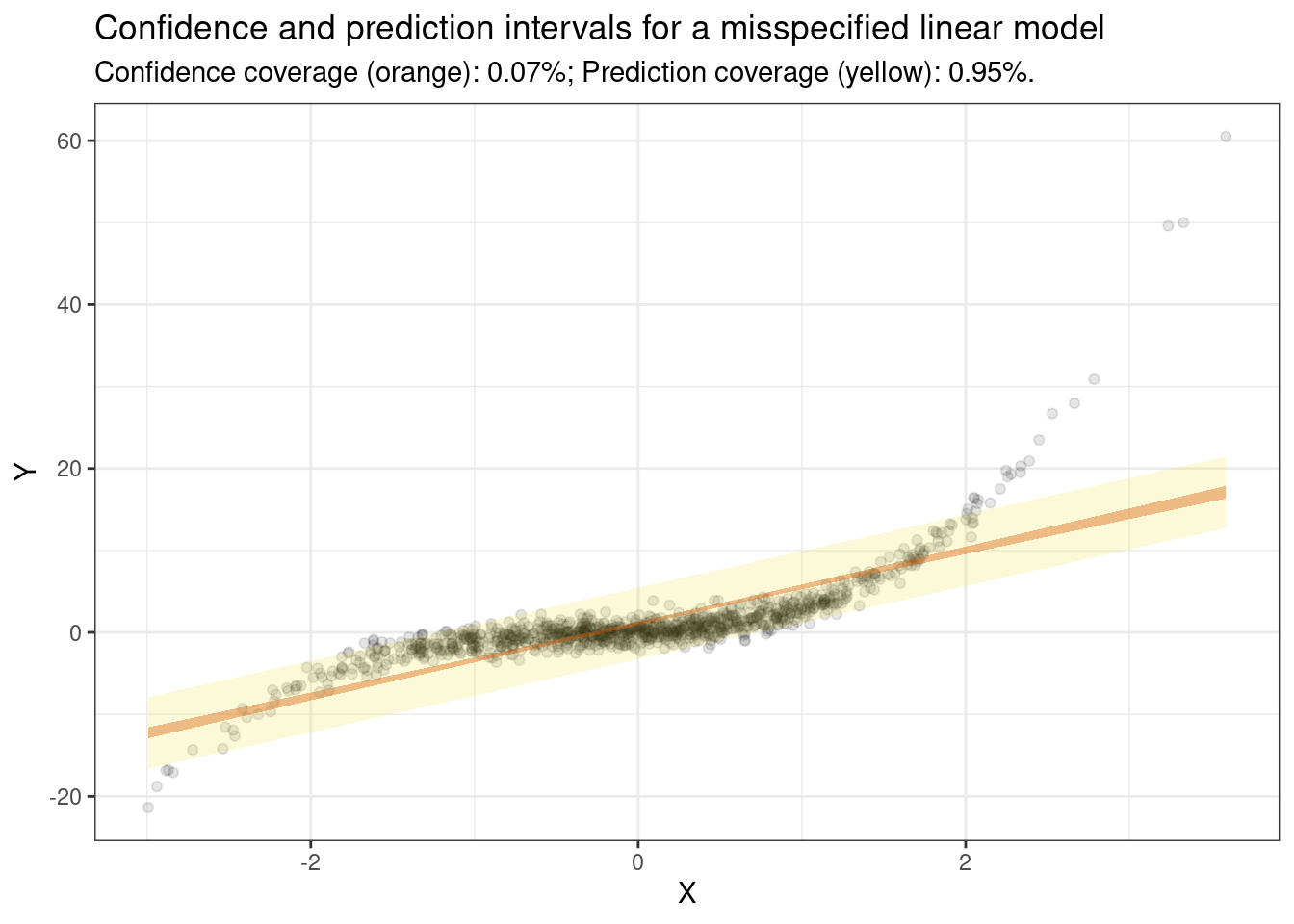
As noted above, the conformal prediction interval should be valid even if the model is misspecified. To illustrate this, we generate data from a linear model with polynomials, but estimate a linear model without polynomials. Then, we plot the results and compute the coverage of the prediction interval:

N <- 1000
X <- rnorm(N * 2)
dat <- data.frame(
    X = X,
    Y = X + X^2 + X^3 + rnorm(N * 2))
train <- dat[1:N,]
test <- dat[(N + 1):nrow(dat),]

m <- lm(Y ~ X, data = train)
p <- predictions(m) |>
    inferences(
        R = 5,
        method = "conformal_cv+",
        conformal_test = test)

mean(p$Y <= p$pred.high & p$Y >= p$pred.low)

[1] 0.953

ggplot(p, aes(X, Y)) +
    geom_point(alpha = .1) +
    geom_ribbon(aes(X, ymin = pred.low, ymax = pred.high), alpha = .2, fill = "#F0E442") +
    geom_ribbon(aes(X, ymin = conf.low, ymax = conf.high), alpha = .4, fill = "#D55E00") +
    theme_bw() +
    labs(
        title = "Confidence and prediction intervals for a misspecified linear model",
        subtitle = sprintf(
            "Confidence coverage (orange): %.2f%%; Prediction coverage (yellow): %.2f%%.",
            mean(p$Y <= p$conf.high & p$Y >= p$conf.low),
            mean(p$Y <= p$pred.high & p$Y >= p$pred.low)))

This example is interesting, because it shows that the prediction interval has adquate marginal coverage. However, the intervals are not necessarily well calibrated “locally”, in different strata of \(X\). In the figure above, our model is misspecified, so we make more mistakes in the tails, where predictions are bad. In contrast, the interval catches more observations in the middle of the distribution, which ensures that the overall error rate is adequate.

Poisson vs Negative Binomial

Here is a second example of model misspecification. We generate data from a negative binomial model, but estimate a Poisson model. Nevertheless, the conformal prediction interval has good coverage:

n <- 10000
X <- rnorm(n)
eta <- -1 + 2*X
mu <- exp(eta)
Y <- rnegbin(n, mu = mu, theta = 1)
dat <- data.frame(X = X, Y = Y)
train <- dat[1:5000,]
test <- dat[5001:nrow(dat),]

mod <- glm(Y ~ X, data = train, family = poisson)

p <- predictions(mod, conf_level = .9) |>
    inferences(
        method = "conformal_cv+",
        R = 10,
        conformal_test = test)

mean(p$Y >= p$pred.low & p$Y <= p$pred.high)

[1] 0.8968

Footnotes

The usual “independent and identically distributed” assumption is a special case of exchangeability.↩︎

Conformal prediction

Confidence vs. prediction intervals

Conformal prediction

Data and models: Linear, Logit, Multinomial Logit

Conformal predictions with inferences()

Cross-validation +

Split conformal prediction

Misspecification

Polynomials

Poisson vs Negative Binomial

Footnotes

Conformal predictions with `inferences()`