library(marginaleffects)

mod <- lm(Sepal.Length ~ Petal.Width * Petal.Length + factor(Species), data = iris)Bootstrap & Simulation
marginaleffects offers an inferences() function to compute uncertainty estimates using the bootstrap and simulation-based inference.
WARNING: The inferences() function is experimental. It may be renamed, the user interface may change, or the functionality may migrate to arguments in other marginaleffects functions.
Consider a simple model:
We will compute uncertainty estimates around the output of comparisons(), but note that the same approach works with the predictions() and slopes() functions as well.
Delta method
The default strategy to compute standard errors and confidence intervals is the delta method. This is what we obtain by calling:
avg_comparisons(mod, by = "Species", variables = "Petal.Width")
#>
#>         Term Contrast    Species Estimate Std. Error      z Pr(>|z|)   S  2.5 % 97.5 %
#>  Petal.Width mean(+1) setosa      -0.1103      0.285 -0.387    0.699 0.5 -0.669  0.449
#>  Petal.Width mean(+1) versicolor  -0.0201      0.160 -0.125    0.900 0.2 -0.334  0.293
#>  Petal.Width mean(+1) virginica    0.0216      0.169  0.128    0.898 0.2 -0.309  0.353
#>
#> Columns: term, contrast, Species, estimate, std.error, statistic, p.value, s.value, conf.low, conf.high, predicted_lo, predicted_hi, predicted
#> Type:  response
Since this is the default method, we obtain the same results if we add the inferences() call in the chain:
avg_comparisons(mod, by = "Species", variables = "Petal.Width") |>
  inferences(method = "delta")
#>
#>         Term Contrast    Species Estimate Std. Error      z Pr(>|z|)   S  2.5 % 97.5 %
#>  Petal.Width mean(+1) setosa      -0.1103      0.285 -0.387    0.699 0.5 -0.669  0.449
#>  Petal.Width mean(+1) versicolor  -0.0201      0.160 -0.125    0.900 0.2 -0.334  0.293
#>  Petal.Width mean(+1) virginica    0.0216      0.169  0.128    0.898 0.2 -0.309  0.353
#>
#> Columns: term, contrast, Species, estimate, std.error, statistic, p.value, s.value, conf.low, conf.high, predicted_lo, predicted_hi, predicted
#> Type:  response
Bootstrap
marginaleffects supports three bootstrap frameworks in R: the well-established boot package, the newer rsample package, and the so-called “bayesian bootstrap” in fwb.
boot
avg_comparisons(mod, by = "Species", variables = "Petal.Width") |>
  inferences(method = "boot")
#>
#>         Term Contrast    Species Estimate Std. Error  2.5 % 97.5 %
#>  Petal.Width mean(+1) setosa      -0.1103      0.273 -0.668  0.391
#>  Petal.Width mean(+1) versicolor  -0.0201      0.169 -0.358  0.302
#>  Petal.Width mean(+1) virginica    0.0216      0.188 -0.363  0.384
#>
#> Columns: term, contrast, Species, estimate, predicted_lo, predicted_hi, predicted, std.error, conf.low, conf.high
#> Type:  response
All unknown arguments that we feed to inferences() are pushed forward to boot::boot():
est <- avg_comparisons(mod, by = "Species", variables = "Petal.Width") |>
  inferences(method = "boot", sim = "balanced", R = 500, conf_type = "bca")
est
#>
#>         Term Contrast    Species Estimate Std. Error  2.5 % 97.5 %
#>  Petal.Width mean(+1) setosa      -0.1103      0.259 -0.667  0.399
#>  Petal.Width mean(+1) versicolor  -0.0201      0.161 -0.305  0.328
#>  Petal.Width mean(+1) virginica    0.0216      0.181 -0.312  0.425
#>
#> Columns: term, contrast, Species, estimate, predicted_lo, predicted_hi, predicted, std.error, conf.low, conf.high
#> Type:  response
We can extract the original boot object from an attribute:
attr(est, "inferences")
#>
#> BALANCED BOOTSTRAP
#>
#>
#> Call:
#> bootstrap_boot(model = model, INF_FUN = INF_FUN, newdata = ..1,
#>     vcov = ..2, variables = ..3, type = ..4, by = ..5, conf_level = ..6,
#>     cross = ..7, comparison = ..8, transform = ..9, wts = ..10,
#>     hypothesis = ..11, eps = ..12)
#>
#>
#> Bootstrap Statistics :
#>        original        bias    std. error
#> t1* -0.11025325  5.954310e-03   0.2587741
#> t2* -0.02006005 -8.021177e-05   0.1610744
#> t3*  0.02158742 -2.866703e-03   0.1813503
Or we can extract the individual draws with the posterior_draws() function:
posterior_draws(est) |> head()
#>   drawid        draw        term contrast    Species    estimate predicted_lo predicted_hi predicted std.error   conf.low conf.high
#> 1      1  0.11930751 Petal.Width mean(+1)     setosa -0.11025325     4.957514     4.845263  4.957514 0.2587741 -0.6673954 0.3992570
#> 2      1  0.13778507 Petal.Width mean(+1) versicolor -0.02006005     6.327949     6.322072  6.327949 0.1610744 -0.3049916 0.3284759
#> 3      1  0.14631724 Petal.Width mean(+1)  virginica  0.02158742     7.015513     7.051542  7.015513 0.1813503 -0.3123242 0.4248907
#> 4      2 -0.02800118 Petal.Width mean(+1)     setosa -0.11025325     4.957514     4.845263  4.957514 0.2587741 -0.6673954 0.3992570
#> 5      2 -0.13140218 Petal.Width mean(+1) versicolor -0.02006005     6.327949     6.322072  6.327949 0.1610744 -0.3049916 0.3284759
#> 6      2 -0.17914846 Petal.Width mean(+1)  virginica  0.02158742     7.015513     7.051542  7.015513 0.1813503 -0.3123242 0.4248907

posterior_draws(est, shape = "DxP") |> dim()
#> [1] 500   3
rsample
As before, we can pass arguments to rsample::bootstraps() through inferences(). For example, for stratified resampling:
est <- avg_comparisons(mod, by = "Species", variables = "Petal.Width") |>
  inferences(method = "rsample", R = 100, strata = "Species")
est
#>
#>         Term Contrast    Species Estimate  2.5 % 97.5 %
#>  Petal.Width mean(+1) setosa      -0.1103 -0.603  0.462
#>  Petal.Width mean(+1) versicolor  -0.0201 -0.383  0.362
#>  Petal.Width mean(+1) virginica    0.0216 -0.410  0.370
#>
#> Columns: term, contrast, Species, estimate, predicted_lo, predicted_hi, predicted, conf.low, conf.high
#> Type:  response

attr(est, "inferences")
#> # Bootstrap sampling using stratification with apparent sample
#> # A tibble: 101 × 3
#>    splits           id           estimates
#>    <list>           <chr>        <list>
#>  1 <split [150/52]> Bootstrap001 <tibble [3 × 7]>
#>  2 <split [150/61]> Bootstrap002 <tibble [3 × 7]>
#>  3 <split [150/54]> Bootstrap003 <tibble [3 × 7]>
#>  4 <split [150/57]> Bootstrap004 <tibble [3 × 7]>
#>  5 <split [150/53]> Bootstrap005 <tibble [3 × 7]>
#>  6 <split [150/57]> Bootstrap006 <tibble [3 × 7]>
#>  7 <split [150/56]> Bootstrap007 <tibble [3 × 7]>
#>  8 <split [150/59]> Bootstrap008 <tibble [3 × 7]>
#>  9 <split [150/56]> Bootstrap009 <tibble [3 × 7]>
#> 10 <split [150/61]> Bootstrap010 <tibble [3 × 7]>
#> # ℹ 91 more rows
Or we can extract the individual draws with the posterior_draws() function:
posterior_draws(est) |> head()
#>   drawid       draw        term contrast    Species    estimate predicted_lo predicted_hi predicted   conf.low conf.high
#> 1      1 0.08180703 Petal.Width mean(+1)     setosa -0.11025325     4.957514     4.845263  4.957514 -0.6034194 0.4618492
#> 2      1 0.17526343 Petal.Width mean(+1) versicolor -0.02006005     6.327949     6.322072  6.327949 -0.3832662 0.3619752
#> 3      1 0.21841770 Petal.Width mean(+1)  virginica  0.02158742     7.015513     7.051542  7.015513 -0.4098139 0.3703826
#> 4      2 0.45231956 Petal.Width mean(+1)     setosa -0.11025325     4.957514     4.845263  4.957514 -0.6034194 0.4618492
#> 5      2 0.35678649 Petal.Width mean(+1) versicolor -0.02006005     6.327949     6.322072  6.327949 -0.3832662 0.3619752
#> 6      2 0.31267330 Petal.Width mean(+1)  virginica  0.02158742     7.015513     7.051542  7.015513 -0.4098139 0.3703826

posterior_draws(est, shape = "PxD") |> dim()
#> [1]   3 100
Fractional Weighted Bootstrap (aka Bayesian Bootstrap)
The fwb package implements fractional weighted bootstrap (aka Bayesian bootstrap):
“fwb implements the fractional weighted bootstrap (FWB), also known as the Bayesian bootstrap, following the treatment by Xu et al. (2020). The FWB involves generating sets of weights from a uniform Dirichlet distribution to be used in estimating statistics of interest, which yields a posterior distribution that can be interpreted in the same way the traditional (resampling-based) bootstrap distribution can be.” -Noah Greifer
The inferences() function makes it easy to apply this inference strategy to marginaleffects objects:
avg_comparisons(mod) |> inferences(method = "fwb")
#>
#>          Term            Contrast Estimate Std. Error  2.5 % 97.5 %
#>  Petal.Length +1                    0.8929     0.0798  0.737  1.054
#>  Petal.Width  +1                   -0.0362     0.1641 -0.344  0.304
#>  Species      versicolor - setosa  -1.4629     0.3255 -2.126 -0.836
#>  Species      virginica - setosa   -1.9842     0.3885 -2.798 -1.255
#>
#> Columns: term, contrast, estimate, std.error, conf.low, conf.high
#> Type:  response
Simulation-based inference
This simulation-based strategy to compute confidence intervals was described in Krinsky & Robb (1986) and popularized by King, Tomz, Wittenberg (2000). We proceed in 3 steps:
- Draw
Rsets of simulated coefficients from a multivariate normal distribution with mean equal to the original model’s estimated coefficients and variance equal to the model’s variance-covariance matrix (classical, “HC3”, or other). - Use the
Rsets of coefficients to computeRsets of estimands: predictions, comparisons, or slopes. - Take quantiles of the resulting distribution of estimands to obtain a confidence interval and the standard deviation of simulated estimates to estimate the standard error.
Here are a few examples:
library(ggplot2)
library(ggdist)

avg_comparisons(mod, by = "Species", variables = "Petal.Width") |>
  inferences(method = "simulation")
#>
#>         Term Contrast    Species Estimate  2.5 % 97.5 %
#>  Petal.Width mean(+1) setosa      -0.1103 -0.657  0.428
#>  Petal.Width mean(+1) versicolor  -0.0201 -0.345  0.293
#>  Petal.Width mean(+1) virginica    0.0216 -0.299  0.349
#>
#> Columns: term, contrast, Species, estimate, predicted_lo, predicted_hi, predicted, conf.low, conf.high
#> Type:  response
Since simulation based inference generates R estimates of the quantities of interest, we can treat them similarly to draws from the posterior distribution in bayesian models. For example, we can extract draws using the posterior_draws() function, and plot their distributions using packages likeggplot2 and ggdist:
avg_comparisons(mod, by = "Species", variables = "Petal.Width") |>
  inferences(method = "simulation") |>
  posterior_draws("rvar") |>
  ggplot(aes(y = Species, xdist = rvar)) +
  stat_slabinterval()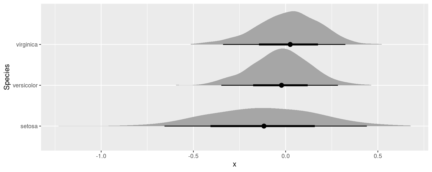
Multiple imputation and missing data
The same workflow and the same inferences function can be used to estimate models with multiple imputation for missing data.