Categorical outcomes
Several packages in the R ecosystem allow users to estimate models for ordered or discrete choice, such as ordered probit or multinomial logit. This case study illustrates the use of marginaleffects with the MASS, nnet, and mlogit packages.
We begin by loading two libraries:
MASS::polr function
Consider a simple ordered logit model in which we predict the number of gears of a car based its miles per gallon and horsepower:
Now, consider a car with 25 miles per gallon and 110 horsepower. The expected predicted probability for each outcome level (gear) for this car is:
predictions(mod, newdata = datagrid(mpg = 25, hp = 110))
#>
#>  Group mpg  hp Estimate Std. Error    z Pr(>|z|)    S  2.5 % 97.5 %
#>      3  25 110    0.203     0.0959 2.12   0.0339  4.9 0.0155  0.391
#>      4  25 110    0.578     0.1229 4.70   <0.001 18.6 0.3373  0.819
#>      5  25 110    0.218     0.1007 2.17   0.0302  5.1 0.0209  0.416
#>
#> Columns: rowid, group, estimate, std.error, statistic, p.value, s.value, conf.low, conf.high, mpg, hp, gear
#> Type:  probs
Since the gear is categorical, we make one prediction for each level of the outcome.
Now consider the marginal effects (aka slopes or partial derivatives) for the same car:
slopes(mod, variables = "mpg", newdata = datagrid(mpg = 25, hp = 110))
#>
#>  Group Term mpg  hp Estimate Std. Error       z Pr(>|z|)    S    2.5 %  97.5 %
#>      3  mpg  25 110 -0.06042     0.0169 -3.5812   <0.001 11.5 -0.09349 -0.0274
#>      4  mpg  25 110 -0.00318     0.0335 -0.0949   0.9244  0.1 -0.06891  0.0625
#>      5  mpg  25 110  0.06361     0.0301  2.1135   0.0346  4.9  0.00462  0.1226
#>
#> Columns: rowid, term, group, estimate, std.error, statistic, p.value, s.value, conf.low, conf.high, mpg, hp, predicted_lo, predicted_hi, predicted, gear
#> Type:  probs
Again, marginaleffects produces one estimate of the slope for each outcome level. For a small step size \(\varepsilon\), the printed quantities are estimated as:
\[\frac{P(gear=3|mpg=25+\varepsilon, hp=110)-P(gear=3|mpg=25-\varepsilon, hp=110)}{2 \cdot \varepsilon}\] \[\frac{P(gear=4|mpg=25+\varepsilon, hp=110)-P(gear=4|mpg=25-\varepsilon, hp=110)}{2 \cdot \varepsilon}\] \[\frac{P(gear=5|mpg=25+\varepsilon, hp=110)-P(gear=5|mpg=25-\varepsilon, hp=110)}{2 \cdot \varepsilon}\]
When we call avg_slopes(), marginaleffects will repeat the same computation for every row of the original dataset, and then report the average slope for each level of the outcome:
avg_slopes(mod)
#>
#>  Group Term Estimate Std. Error     z Pr(>|z|)    S     2.5 %   97.5 %
#>      3  hp  -0.00377   0.001514 -2.49  0.01285  6.3 -0.006735 -0.00080
#>      3  mpg -0.07014   0.015483 -4.53  < 0.001 17.4 -0.100485 -0.03979
#>      4  hp   0.00201   0.000958  2.10  0.03554  4.8  0.000136  0.00389
#>      4  mpg  0.03748   0.013860  2.70  0.00685  7.2  0.010311  0.06464
#>      5  hp   0.00175   0.000833  2.11  0.03518  4.8  0.000122  0.00339
#>      5  mpg  0.03266   0.009570  3.41  < 0.001 10.6  0.013905  0.05142
#>
#> Columns: term, group, estimate, std.error, statistic, p.value, s.value, conf.low, conf.high
#> Type:  probs
nnet package
The multinom function of the nnet package allows users to fit log-linear models via neural networks. The data used for this function is a data frame with one observation per row, and the response variable is coded a factor. All the marginaleffects package function work seamlessly with this model. For example, we can estimate a model and compute average marginal effects as follows:
library(nnet)

head(mtcars)
#>                    mpg cyl disp  hp drat    wt  qsec vs am gear carb
#> Mazda RX4         21.0   6  160 110 3.90 2.620 16.46  0  1    4    4
#> Mazda RX4 Wag     21.0   6  160 110 3.90 2.875 17.02  0  1    4    4
#> Datsun 710        22.8   4  108  93 3.85 2.320 18.61  1  1    4    1
#> Hornet 4 Drive    21.4   6  258 110 3.08 3.215 19.44  1  0    3    1
#> Hornet Sportabout 18.7   8  360 175 3.15 3.440 17.02  0  0    3    2
#> Valiant           18.1   6  225 105 2.76 3.460 20.22  1  0    3    1

mod <- multinom(factor(gear) ~ hp + mpg, data = mtcars, trace = FALSE)

avg_slopes(mod, type = "probs")
#>
#>  Group Term  Estimate Std. Error       z Pr(>|z|)    S    2.5 %    97.5 %
#>      3  hp  -3.36e-05    0.00225 -0.0149  0.98809  0.0 -0.00444  0.004372
#>      3  mpg -7.13e-02    0.02646 -2.6951  0.00704  7.2 -0.12315 -0.019448
#>      4  hp  -4.67e-03    0.00221 -2.1126  0.03463  4.9 -0.00900 -0.000337
#>      4  mpg  1.59e-02    0.02010  0.7917  0.42851  1.2 -0.02348  0.055316
#>      5  hp   4.70e-03    0.00130  3.6170  < 0.001 11.7  0.00215  0.007247
#>      5  mpg  5.54e-02    0.01642  3.3732  < 0.001 10.4  0.02320  0.087563
#>
#> Columns: term, group, estimate, std.error, statistic, p.value, s.value, conf.low, conf.high
#> Type:  probs
Notice that in such models, we get one marginal effect for each term, for each level of the response variable. For this reason, we should use "group" in the condition argument (or facet_*() function) when calling one of the plotting functions:
library(ggplot2)

plot_predictions(mod, condition = c("mpg", "group"), type = "probs")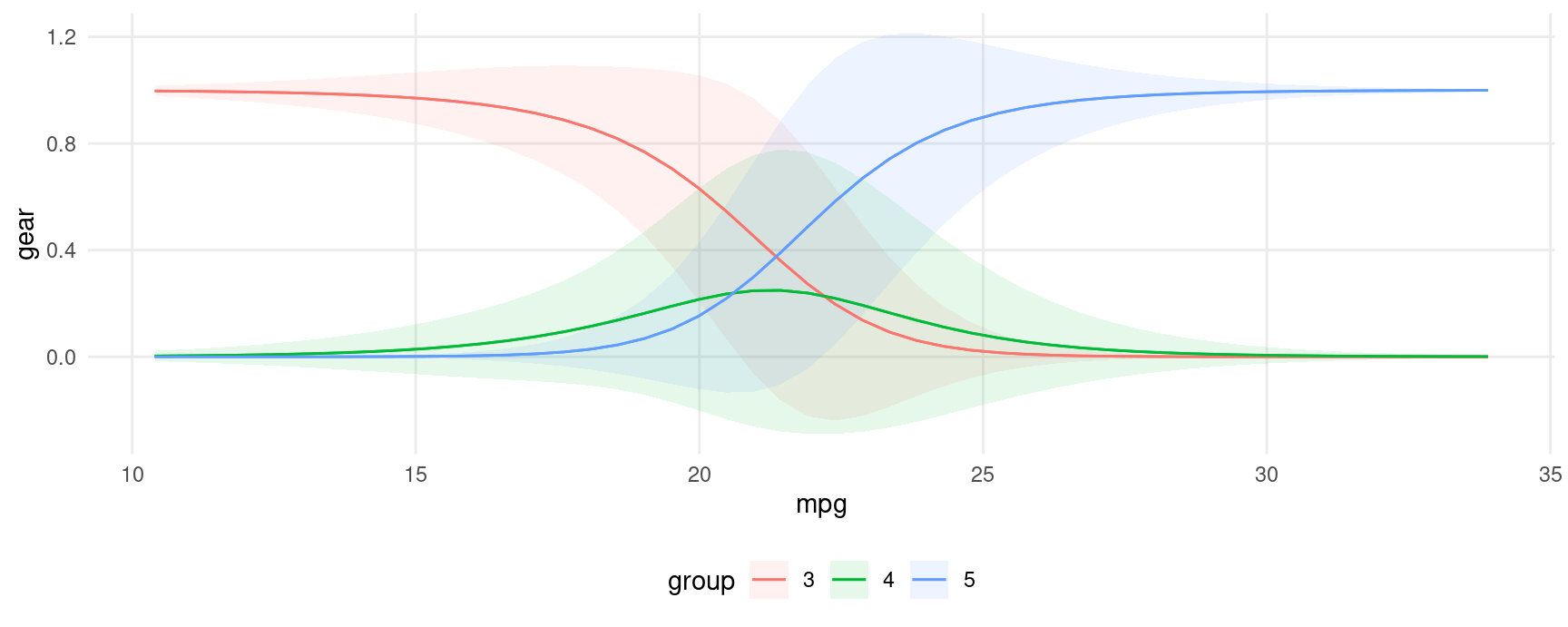
plot_predictions(mod, condition = "mpg", type = "probs") + facet_wrap(~group)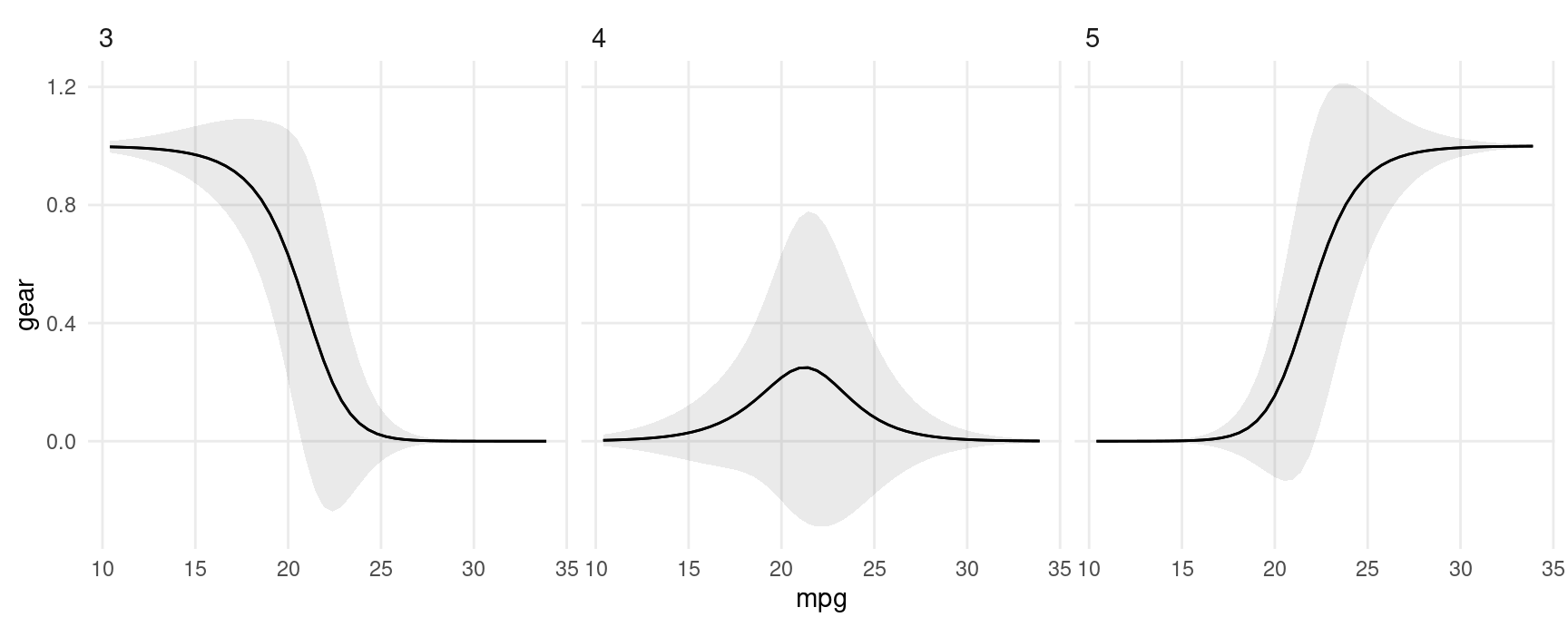
plot_comparisons(
    mod,
    variables = list(mpg = c(15, 30)),
    condition = "group",
    type = "probs")
mlogit package
The mlogit package uses data in a slightly different structure, with one row per observation-choice combination. For example, this data on choice of travel mode includes 4 rows per individual, one for each mode of transportation:
library("AER")
library("mlogit")
library("tidyverse")
data("TravelMode", package = "AER")

head(TravelMode)
#>   individual  mode choice wait vcost travel gcost income size
#> 1          1   air     no   69    59    100    70     35    1
#> 2          1 train     no   34    31    372    71     35    1
#> 3          1   bus     no   35    25    417    70     35    1
#> 4          1   car    yes    0    10    180    30     35    1
#> 5          2   air     no   64    58     68    68     30    2
#> 6          2 train     no   44    31    354    84     30    2

mod <- mlogit(choice ~ wait + gcost | income + size, TravelMode)

avg_slopes(mod, variables = c("income", "size"))
#>
#>  Group   Term  Estimate Std. Error      z Pr(>|z|)    S     2.5 %   97.5 %
#>  air   income  0.002786    0.00122  2.289  0.02209  5.5  0.000400  0.00517
#>  air   size   -0.126477    0.02892 -4.373  < 0.001 16.3 -0.183162 -0.06979
#>  bus   income -0.000372    0.00110 -0.338  0.73557  0.4 -0.002531  0.00179
#>  bus   size    0.011349    0.02587  0.439  0.66084  0.6 -0.039347  0.06204
#>  car   income  0.003373    0.00137  2.455  0.01407  6.2  0.000681  0.00607
#>  car   size    0.045887    0.02476  1.853  0.06381  4.0 -0.002636  0.09441
#>  train income -0.005787    0.00132 -4.390  < 0.001 16.4 -0.008371 -0.00320
#>  train size    0.069241    0.02478  2.794  0.00521  7.6  0.020666  0.11782
#>
#> Columns: term, group, estimate, std.error, statistic, p.value, s.value, conf.low, conf.high
#> Type:  response
Note that the slopes function will always return estimates of zero for regressors before the vertical bar in the formula. This is because marginaleffects increments all rows of the prediction dataset in the same way to compute slopes and contrast. Because mlogit data are in “long” format, this means that alternatives are incremented in the same way, which does not produce alternative-specific changes in the predictors.
One strategy to circumvent this problem is to supply a data frame of numeric values to compare, with alternative specific changes. In this example, we test what happens to the probability of selecting each mode of transportation if we only increase the wait time of air travel:
altspec <- data.frame(
  low = TravelMode$wait,
  high = ifelse(TravelMode$mode == "air", TravelMode$wait + 15, TravelMode$wait)
)

avg_comparisons(mod, variables = list(wait = altspec))
#>
#>  Group Term Contrast Estimate Std. Error      z Pr(>|z|)     S   2.5 %  97.5 %
#>  air   wait   manual  -0.1321    0.01070 -12.35   <0.001 114.0 -0.1531 -0.1111
#>  bus   wait   manual   0.0251    0.00460   5.45   <0.001  24.2  0.0160  0.0341
#>  car   wait   manual   0.0701    0.00834   8.41   <0.001  54.5  0.0538  0.0865
#>  train wait   manual   0.0369    0.00528   6.99   <0.001  38.4  0.0266  0.0473
#>
#> Columns: term, group, contrast, estimate, std.error, statistic, p.value, s.value, conf.low, conf.high
#> Type:  response
We can compute yet more kinds of marginal effects, we can construct customized data frames and feed them to the newdata argument of the slopes function.
If we want to compute the slope of the response function (marginal effects) when each of the predictors is fixed to its global mean, we can do:
nd <- TravelMode |>
    summarize(across(c("wait", "gcost", "income", "size"),
              function(x) rep(mean(x), 4)))
nd
#>       wait    gcost   income     size
#> 1 34.58929 110.8798 34.54762 1.742857
#> 2 34.58929 110.8798 34.54762 1.742857
#> 3 34.58929 110.8798 34.54762 1.742857
#> 4 34.58929 110.8798 34.54762 1.742857

avg_slopes(mod, newdata = nd, variables = c("income", "size"))
#>
#>  Group   Term  Estimate Std. Error     z Pr(>|z|)   S     2.5 %    97.5 %
#>  air   income  6.66e-03   2.42e-03  2.75  0.00599 7.4  1.91e-03  1.14e-02
#>  air   size   -1.69e-01   5.87e-02 -2.88  0.00393 8.0 -2.85e-01 -5.43e-02
#>  bus   income -1.14e-03   9.43e-04 -1.21  0.22630 2.1 -2.99e-03  7.07e-04
#>  bus   size    4.67e-02   2.72e-02  1.72  0.08622 3.5 -6.65e-03  1.00e-01
#>  car   income  6.48e-06   2.02e-05  0.32  0.74885 0.4 -3.32e-05  4.62e-05
#>  car   size    1.36e-03   8.81e-04  1.54  0.12304 3.0 -3.68e-04  3.08e-03
#>  train income -5.52e-03   1.91e-03 -2.89  0.00384 8.0 -9.27e-03 -1.78e-03
#>  train size    1.21e-01   4.44e-02  2.73  0.00634 7.3  3.42e-02  2.08e-01
#>
#> Columns: term, group, estimate, std.error, statistic, p.value, s.value, conf.low, conf.high
#> Type:  response
If we want to compute marginal effects with the gcost and wait fixed at their mean value, conditional on the choice of transportation mode:
nd <- TravelMode |>
    group_by(mode) |>
    summarize(across(c("wait", "gcost", "income", "size"), mean))
nd
#> # A tibble: 4 × 5
#>   mode   wait gcost income  size
#>   <fct> <dbl> <dbl>  <dbl> <dbl>
#> 1 air    61.0 103.    34.5  1.74
#> 2 train  35.7 130.    34.5  1.74
#> 3 bus    41.7 115.    34.5  1.74
#> 4 car     0    95.4   34.5  1.74

avg_slopes(mod, newdata = nd, variables = c("income", "size"))
#>
#>  Group   Term  Estimate Std. Error      z Pr(>|z|)    S     2.5 %   97.5 %
#>  air   income  0.006015    0.00233  2.587  0.00968  6.7  0.001458  0.01057
#>  air   size   -0.232955    0.05661 -4.115  < 0.001 14.7 -0.343900 -0.12201
#>  bus   income -0.000713    0.00146 -0.489  0.62478  0.7 -0.003568  0.00214
#>  bus   size    0.020447    0.03436  0.595  0.55185  0.9 -0.046906  0.08780
#>  car   income  0.005445    0.00229  2.382  0.01724  5.9  0.000964  0.00993
#>  car   size    0.067839    0.04123  1.645  0.09991  3.3 -0.012974  0.14865
#>  train income -0.010748    0.00256 -4.201  < 0.001 15.2 -0.015762 -0.00573
#>  train size    0.144669    0.04773  3.031  0.00244  8.7  0.051127  0.23821
#>
#> Columns: term, group, estimate, std.error, statistic, p.value, s.value, conf.low, conf.high
#> Type:  response
We can also explore more complex alternatives. Here, for example, only one alternative is affected by cost reduction:
nd <- datagrid(mode = TravelMode$mode, newdata = TravelMode)
nd <- lapply(1:4, function(i) mutate(nd, gcost = ifelse(1:4 == i, 30, gcost)))
nd <- bind_rows(nd)
nd
#>    individual choice wait vcost travel gcost income size  mode rowid
#> 1           1     no   35    48    486    30     35    2   air     1
#> 2           1     no   35    48    486   111     35    2 train     2
#> 3           1     no   35    48    486   111     35    2   bus     3
#> 4           1     no   35    48    486   111     35    2   car     4
#> 5           1     no   35    48    486   111     35    2   air     1
#> 6           1     no   35    48    486    30     35    2 train     2
#> 7           1     no   35    48    486   111     35    2   bus     3
#> 8           1     no   35    48    486   111     35    2   car     4
#> 9           1     no   35    48    486   111     35    2   air     1
#> 10          1     no   35    48    486   111     35    2 train     2
#> 11          1     no   35    48    486    30     35    2   bus     3
#> 12          1     no   35    48    486   111     35    2   car     4
#> 13          1     no   35    48    486   111     35    2   air     1
#> 14          1     no   35    48    486   111     35    2 train     2
#> 15          1     no   35    48    486   111     35    2   bus     3
#> 16          1     no   35    48    486    30     35    2   car     4

avg_slopes(mod, newdata = nd, variables = c("income", "size"))
#>
#>  Group   Term  Estimate Std. Error      z Pr(>|z|)    S     2.5 %    97.5 %
#>  air   income  8.24e-03   2.46e-03  3.352   <0.001 10.3  3.42e-03  0.013058
#>  air   size   -2.12e-01   6.02e-02 -3.526   <0.001 11.2 -3.30e-01 -0.094353
#>  bus   income -1.33e-03   1.30e-03 -1.020    0.308  1.7 -3.88e-03  0.001223
#>  bus   size    6.06e-02   3.79e-02  1.600    0.110  3.2 -1.36e-02  0.134895
#>  car   income  2.66e-05   4.31e-05  0.617    0.537  0.9 -5.78e-05  0.000111
#>  car   size    2.38e-03   1.57e-03  1.512    0.131  2.9 -7.04e-04  0.005459
#>  train income -6.94e-03   1.86e-03 -3.735   <0.001 12.4 -1.06e-02 -0.003298
#>  train size    1.49e-01   4.28e-02  3.488   <0.001 11.0  6.55e-02  0.233374
#>
#> Columns: term, group, estimate, std.error, statistic, p.value, s.value, conf.low, conf.high
#> Type:  response
Important: The newdata argument for mlogit models must be a “balanced” data frame, that is, it must have a number of rows that is a multiple of the number of choices.