Style

The main styling function for the tinytable package is style_tt(). Via this function, you can access three main interfaces to customize tables:

1. A general interface to frequently used style choices which works for both HTML and LaTeX (PDF): colors, font style and size, row and column spans, etc. This is accessed through several distinct arguments in the style_tt() function, such as italic, color, etc.
2. A specialized interface which allows users to use the powerful tabularray package to customize LaTeX tables. This is accessed by passing tabularray settings as strings to the inner and outer arguments of theme_latex().
3. A specialized interface which allows users to use the powerful Bootstrap framework to customize HTML tables. This is accessed by passing CSS declarations and rules to the bootstrap_css and bootstrap_css_rule arguments of style_tt().

These functions can be used to customize rows, columns, or individual cells. They control many features, including:

• Text color
• Background color
• Widths
• Heights
• Alignment
• Text Wrapping
• Column and Row Spacing
• Cell Merging
• Multi-row or column spans
• Border Styling
• Font Styling: size, underline, italic, bold, strikethrough, etc.
• Header Customization

The style_*() functions can modify individual cells, or entire columns and rows. The portion of the table that is styled is determined by the i (rows) and j (columns) arguments.

library(tinytable)
options(tinytable_tt_digits = 3)
options(tinytable_latex_placement = "H")
x <- mtcars[1:4, 1:5]

Cells, rows, columns

To style individual cells, we use the style_cell() function. The first two arguments—i and j—identify the cells of interest, by row and column numbers respectively. To style a cell in the 2nd row and 3rd column, we can do:

tt(x) |>
  style_tt(
    i = 2,
    j = 3,
    background = "black",
    color = "white"
  )

mpg	cyl	disp	hp	drat
21	6	160	110	3.9
21	6	160	110	3.9
22.8	4	108	93	3.85
21.4	6	258	110	3.08

The i and j accept vectors of integers to modify several cells at once:

tt(x) |>
  style_tt(
    i = 2:3,
    j = c(1, 3, 4),
    italic = TRUE,
    color = "orange"
  )

mpg	cyl	disp	hp	drat
21	6	160	110	3.9
21	6	160	110	3.9
22.8	4	108	93	3.85
21.4	6	258	110	3.08

We can style all cells in a table by omitting both the i and j arguments:

tt(x) |> style_tt(color = "orange")

mpg	cyl	disp	hp	drat
21	6	160	110	3.9
21	6	160	110	3.9
22.8	4	108	93	3.85
21.4	6	258	110	3.08

We can style entire rows by omitting the j argument:

tt(x) |> style_tt(i = 1:2, color = "orange")

mpg	cyl	disp	hp	drat
21	6	160	110	3.9
21	6	160	110	3.9
22.8	4	108	93	3.85
21.4	6	258	110	3.08

We can style entire columns by omitting the i argument:

tt(x) |> style_tt(j = c(2, 4), bold = TRUE)

mpg	cyl	disp	hp	drat
21	6	160	110	3.9
21	6	160	110	3.9
22.8	4	108	93	3.85
21.4	6	258	110	3.08

The j argument accepts integer vectors, character vectors, but also a string with a Perl-style regular expression, which makes it easier to select columns by name:

tt(x) |> style_tt(j = c("mpg", "drat"), color = "orange")

mpg	cyl	disp	hp	drat
21	6	160	110	3.9
21	6	160	110	3.9
22.8	4	108	93	3.85
21.4	6	258	110	3.08

tt(x) |> style_tt(j = "mpg|drat", color = "orange")

mpg	cyl	disp	hp	drat
21	6	160	110	3.9
21	6	160	110	3.9
22.8	4	108	93	3.85
21.4	6	258	110	3.08

Here we use a “negative lookahead” to exclude certain columns:

tt(x) |> style_tt(j = "^(?!drat|mpg)", color = "orange")

mpg	cyl	disp	hp	drat
21	6	160	110	3.9
21	6	160	110	3.9
22.8	4	108	93	3.85
21.4	6	258	110	3.08

Of course, we can also call the style_tt() function several times to apply different styles to different parts of the table:

tt(x) |>
  style_tt(i = 1, j = 1:2, color = "orange") |>
  style_tt(i = 1, j = 3:4, color = "green")

mpg	cyl	disp	hp	drat
21	6	160	110	3.9
21	6	160	110	3.9
22.8	4	108	93	3.85
21.4	6	258	110	3.08

The i argument also accepts unquoted expressions for non-standard evaluation. This allows us to style rows based on data conditions:

tt(x) |> 
  style_tt(i = mpg > 21, background = "lightblue", bold = TRUE)

mpg	cyl	disp	hp	drat
21	6	160	110	3.9
21	6	160	110	3.9
22.8	4	108	93	3.85
21.4	6	258	110	3.08

There is also a groupi object with indices that can be manipulated as an unquoted numeric expression.

tt(head(mtcars, 10)) |>
    group_tt(i = list("Hello" = 3, "World" = 5)) |>
    group_tt(j = list("Cyl" = 1:3, "Disp" = 4:6)) |>
    style_tt(groupi, background = "pink", align = "c") |>
    style_tt(groupi + 1, color = "white", background = "teal")

Cyl			Disp
mpg	cyl	disp	hp	drat	wt	qsec	vs	am	gear	carb
21	6	160	110	3.9	2.62	16.5	0	1	4	4
21	6	160	110	3.9	2.88	17	0	1	4	4
Hello	Hello	Hello	Hello	Hello	Hello	Hello	Hello	Hello	Hello	Hello
22.8	4	108	93	3.85	2.32	18.6	1	1	4	1
21.4	6	258	110	3.08	3.21	19.4	1	0	3	1
World	World	World	World	World	World	World	World	World	World	World
18.7	8	360	175	3.15	3.44	17	0	0	3	2
18.1	6	225	105	2.76	3.46	20.2	1	0	3	1
14.3	8	360	245	3.21	3.57	15.8	0	0	3	4
24.4	4	147	62	3.69	3.19	20	1	0	4	2
22.8	4	141	95	3.92	3.15	22.9	1	0	4	2
19.2	6	168	123	3.92	3.44	18.3	1	0	4	4

Colors

The color and background arguments in the style_tt() function are used for specifying the text color and the background color for cells of a table created by the tt() function. This argument plays a crucial role in enhancing the visual appeal and readability of the table, whether it’s rendered in LaTeX or HTML format. The way we specify colors differs slightly between the two formats:

For HTML Output:

• Hex Codes: You can specify colors using hexadecimal codes, which consist of a # followed by 6 characters (e.g., #CC79A7). This allows for a wide range of colors.
• Keywords: There’s also the option to use color keywords for convenience. The supported keywords are basic color names like black, red, blue, etc.

For LaTeX Output:

• Hexadecimal Codes: Similar to HTML, you can use hexadecimal codes.
• Keywords: LaTeX supports a different set of color keywords, which include standard colors like black, red, blue, as well as additional ones like cyan, darkgray, lightgray, etc.
• Color Blending: An advanced feature in LaTeX is color blending, which can be achieved using the xcolor package. You can blend colors by specifying ratios (e.g., white!80!blue or green!20!red).
• Luminance Levels: The ninecolors package in LaTeX offers colors with predefined luminance levels, allowing for more nuanced color choices (e.g., “azure4”, “magenta8”).

Note that the keywords used in LaTeX and HTML are slightly different.

tt(x) |> style_tt(i = 1:4, j = 1, color = "#FF5733")

mpg	cyl	disp	hp	drat
21	6	160	110	3.9
21	6	160	110	3.9
22.8	4	108	93	3.85
21.4	6	258	110	3.08

Note that when using Hex codes in a LaTeX table, we need extra declarations in the LaTeX preamble. See ?tt for details.

Alignment

To align columns, we use a single character, or a string where each letter represents a column:

dat <- data.frame(
  a = c("a", "aaa", "aaaaa"),
  b = c("b", "bbb", "bbbbb"),
  c = c("c", "ccc", "ccccc")
)

tt(dat) |> style_tt(j = 1:3, align = "c")

a	b	c
a	b	c
aaa	bbb	ccc
aaaaa	bbbbb	ccccc

tt(dat) |> style_tt(j = 1:3, align = "lcr")

a	b	c
a	b	c
aaa	bbb	ccc
aaaaa	bbbbb	ccccc

In LaTeX documents (only), we can use decimal-alignment:

z <- data.frame(pi = c(pi * 100, pi * 1000, pi * 10000, pi * 100000))
tt(z) |>
  format_tt(j = 1, digits = 8, num_fmt = "significant_cell") |>
  style_tt(j = 1, align = "d")

pi
314.15927
3141.5927
31415.927
314159.27

Font size

The font size is specified in em units.

tt(x) |> style_tt(i = 1:4, j = "mpg|hp|qsec", fontsize = 1.5)

mpg	cyl	disp	hp	drat
21	6	160	110	3.9
21	6	160	110	3.9
22.8	4	108	93	3.85
21.4	6	258	110	3.08

Spanning cells (merging cells)

Sometimes, it can be useful to make a cell stretch across multiple colums or rows, for example when we want to insert a label. To achieve this, we can use the colspan argument. Here, we make the 2nd cell of the 2nd row stretch across three columns and two rows:

tt(x) |> style_tt(
  i = 2, j = 2,
  colspan = 3,
  rowspan = 2,
  align = "c",
  alignv = "m",
  color = "white",
  background = "black",
  bold = TRUE
)

mpg	cyl	disp	hp	drat
21	6	160	110	3.9
21	6	160	110	3.9
22.8	4	108	93	3.85
21.4	6	258	110	3.08

Here is the original table for comparison:

tt(x)

mpg	cyl	disp	hp	drat
21	6	160	110	3.9
21	6	160	110	3.9
22.8	4	108	93	3.85
21.4	6	258	110	3.08

Spanning cells can be particularly useful when we want to suppress redundant labels:

tab <- aggregate(mpg ~ cyl + am, FUN = mean, data = mtcars)
tab <- tab[order(tab$cyl, tab$am), ]
tab

  cyl am      mpg
1   4  0 22.90000
4   4  1 28.07500
2   6  0 19.12500
5   6  1 20.56667
3   8  0 15.05000
6   8  1 15.40000

tt(tab, digits = 2) |>
  style_tt(i = c(1, 3, 5), j = 1, rowspan = 2, alignv = "t")

cyl	am	mpg
4	0	23
4	1	28
6	0	19
6	1	21
8	0	15
8	1	15

The rowspan feature is also useful to create multi-row labels. For example, in this table there is a linebreak, but all the text fits in a single cell:

tab <- data.frame(Letters = c("A<br>B", ""), Numbers = c("First", "Second"))

tt(tab) |>
  theme_html(class = "table-bordered")

Letters	Numbers
A B	First
	Second

Now, we use colspan to ensure that that cells in the first column take up less space and are combined into one:

tt(tab) |>
  theme_html(class = "table-bordered") |>
  style_tt(1, 1, rowspan = 2)

Letters	Numbers
A B	First
	Second

We can combine several spans to create complex tables like this one:

df <- structure(list(
  Col1 = c("Col Header", "Item 0", "Item 1", "Item 2", "Total"), 
  Col2 = c("Span 1", "X", "xx", "xx", "xxxx"), 
  Col2.1 = c("Span 1", "Y", "xx", "xx", "xxxx"), 
  Col2.2 = c("Span 2", "X", "xx", "xx", "xxxx"), 
  Col2.3 = c("Span 2", "Y", "xx", "xx", "xxxx")), 
  class = "data.frame", row.names = c(NA, -5L))
df |>
    setNames(NULL) |>
    tt() |>
    style_tt(1, 1, rowspan = 2, bold = TRUE) |>
    style_tt(1, c(2, 4), colspan = 2, bold = TRUE) |>
    style_tt(5, c(2, 4), colspan = 2) |>
    theme_grid()

Col Header	Span 1	Span 1	Span 2	Span 2
Item 0	X	Y	X	Y
Item 1	xx	xx	xx	xx
Item 2	xx	xx	xx	xx
Total	xxxx	xxxx	xxxx	xxxx

Headers

The header can be omitted from the table by using the colnames argument.

tt(x, colnames = FALSE)

21	6	160	110	3.9
21	6	160	110	3.9
22.8	4	108	93	3.85
21.4	6	258	110	3.08

The first is row 0, and higher level headers (ex: column spanning labels) have negative indices like -1. They can be styled as expected:

tt(x) |> style_tt(i = 0, color = "white", background = "black")

mpg	cyl	disp	hp	drat
21	6	160	110	3.9
21	6	160	110	3.9
22.8	4	108	93	3.85
21.4	6	258	110	3.08

When styling columns without specifying i, the headers are styled in accordance with the rest of the column:

tt(x) |> style_tt(j = 2:3, color = "white", background = "black")

mpg	cyl	disp	hp	drat
21	6	160	110	3.9
21	6	160	110	3.9
22.8	4	108	93	3.85
21.4	6	258	110	3.08

Conditional styling

We can use the standard which function from Base R to create indices and apply conditional stying on rows. And we can use a regular expression in j to apply conditional styling on columns:

k <- mtcars[1:10, c("mpg", "am", "vs")]

tt(k) |>
  style_tt(
    i = which(k$am == k$vs),
    j = "am|vs",
    background = "teal",
    color = "white"
  )

mpg	am	vs
21	1	0
21	1	0
22.8	1	1
21.4	0	1
18.7	0	0
18.1	0	1
14.3	0	0
24.4	0	1
22.8	0	1
19.2	0	1

We can also use non-standard evaluation to apply conditional styling directly with unquoted expressions:

tt(k) |>
  style_tt(i = mpg > 22, background = "lightgreen", bold = TRUE)

mpg	am	vs
21	1	0
21	1	0
22.8	1	1
21.4	0	1
18.7	0	0
18.1	0	1
14.3	0	0
24.4	0	1
22.8	0	1
19.2	0	1

Users can also supply a logical matrix of the same size as x to indicate which cell should be styled. For example, we can change the colors of certain entries in a correlation matrix as follows:

cormat <- data.frame(cor(mtcars[1:5]))
tt(cormat, digits = 2) |>
  style_tt(i = abs(cormat) > .8, background = "black", color = "white")

mpg	cyl	disp	hp	drat
1	-0.85	-0.85	-0.78	0.68
-0.85	1	0.9	0.83	-0.7
-0.85	0.9	1	0.79	-0.71
-0.78	0.83	0.79	1	-0.45
0.68	-0.7	-0.71	-0.45	1

Vectorized styling (heatmaps)

The color, background, and fontsize arguments are vectorized. This allows easy specification of different colors in a single call:

tt(x) |>
  style_tt(
    i = 1:4,
    color = c("red", "blue", "green", "orange")
  )

mpg	cyl	disp	hp	drat
21	6	160	110	3.9
21	6	160	110	3.9
22.8	4	108	93	3.85
21.4	6	258	110	3.08

When using a single value for a vectorized argument, it gets applied to all values:

tt(x) |>
  style_tt(
    j = 2:3,
    color = c("orange", "green"),
    background = "black"
  )

mpg	cyl	disp	hp	drat
21	6	160	110	3.9
21	6	160	110	3.9
22.8	4	108	93	3.85
21.4	6	258	110	3.08

We can also produce more complex heatmap-like tables to illustrate different font sizes in em units:

# font sizes
fs <- seq(.1, 2, length.out = 20)

# headless table
k <- data.frame(matrix(fs, ncol = 5))

# colors
bg <- hcl.colors(20, "Inferno")
fg <- ifelse(as.matrix(k) < 1.7, tail(bg, 1), head(bg, 1))

# table
tt(k, width = .7, theme = "empty", colnames = FALSE) |>
  style_tt(j = 1:5, align = "ccccc", alignv = "m") |>
  style_tt(
    i = 1:4,
    j = 1:5,
    color = fg,
    background = bg,
    fontsize = fs
  )

0.1	0.5	0.9	1.3	1.7
0.2	0.6	1	1.4	1.8
0.3	0.7	1.1	1.5	1.9
0.4	0.8	1.2	1.6	2

Lines (borders)

The style_tt function allows us to customize the borders that surround eacell of a table, as well horizontal and vertical rules. To control these lines, we use the line, line_width, and line_color arguments. Here’s a brief overview of each of these arguments:

• line: This argument specifies where solid lines should be drawn. It is a string that can consist of the following characters:
  • "t": Draw a line at the top of the cell, row, or column.
  • "b": Draw a line at the bottom of the cell, row, or column.
  • "l": Draw a line at the left side of the cell, row, or column.
  • "r": Draw a line at the right side of the cell, row, or column.
  • You can combine these characters to draw lines on multiple sides, such as "tbl" to draw lines at the top, bottom, and left sides of a cell.
• line_width: This argument controls the width of the solid lines in em units (default: 0.1 em). You can adjust this value to make the lines thicker or thinner.
• line_color: Specifies the color of the solid lines. You can use color names, hexadecimal codes, or other color specifications to define the line color.

Here is an example where we draw lines around every border (“t”, “b”, “l”, and “r”) of specified cells.

tt(x, theme = "empty") |>
  style_tt(
    i = 0:3,
    j = 1:3,
    line = "tblr",
    line_width = 0.4,
    line_color = "orange"
  )

mpg	cyl	disp	hp	drat
21	6	160	110	3.9
21	6	160	110	3.9
22.8	4	108	93	3.85
21.4	6	258	110	3.08

And here is an example with horizontal rules:

tt(x, theme = "empty") |>
  style_tt(i = 0, line = "t", line_color = "orange", line_width = 0.4) |>
  style_tt(i = 1, line = "t", line_color = "purple", line_width = 0.2) |>
  style_tt(i = 4, line = "b", line_color = "orange", line_width = 0.4)

mpg	cyl	disp	hp	drat
21	6	160	110	3.9
21	6	160	110	3.9
22.8	4	108	93	3.85
21.4	6	258	110	3.08

dat <- data.frame(1:2, 3:4, 5:6, 7:8)

tt(dat, theme = "empty", colnames = FALSE) |>
  style_tt(
    line = "tblr", line_color = "white", line_width = 0.5,
    background = "blue", color = "white"
  )

1	3	5	7
2	4	6	8

Markdown

Markdown is a text-only format with limited styling options. The only supported arguments are: bold, italic, and strikeout. These limitations exist because there is no standard markdown syntax for other styling options (ex: colors and background).

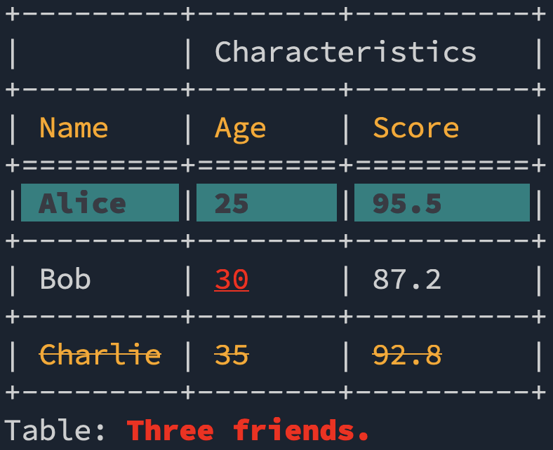
However, in terminals (consoles) that support it, tinytable can display colors and text styles using ANSI escape codes by setting theme_markdown(ansi = TRUE). This allows for rich formatting in compatible terminal environments.

Here’s an example with multiple ANSI styles:

data <- data.frame(
  Name = c("Alice", "Bob", "Charlie"),
  Age = c(25, 30, 35),
  Score = c(95.5, 87.2, 92.8)
)

tt(data, caption = "Three friends.") |>
  style_tt(i = c(0, 3), color = "orange") |>
  style_tt(i = 1, background = "teal", color = "black", bold = TRUE) |>
  style_tt(i = 2, j = 2, underline = TRUE, color = "red") |>
  style_tt(i = 3, strikeout = TRUE) |>
  group_tt(j = list("Characteristics" = 2:3)) |>
  style_tt(i = "caption", bold = TRUE, color = "red") |>
  theme_markdown(ansi = TRUE)

ANSI Terminal Output