Interactive tables

Experimental and Evolving Feature

The Tabulator.js integration is experimental and the API may change in future versions. Please report any issues on GitHub.

Version Requirement

This vignette was compiled using tinytable version 0.14.0.7. Some features shown here may not be available in the CRAN version of tinytable.

Get the development version at:

library(remotes)
install_github("vincentarelbundock/tinytable")

Make sure you restart R for the install to take effect.

The tinytable package supports creating interactive tables using the Tabulator.js library. Tabulator is a powerful JavaScript library that provides features like

Sorting
Filtering
Pagination
Themes
Data export
Real-time data editing in the browser
Accessibility features (ARIA compliant)

Drawing, printing, and saving

To create an interactive table, use the theme_html(engine="tabulator") function:

library(tinytable)
dat <- head(iris)
tt(dat) |> 
  theme_html(engine = "tabulator") |> 
  print("html")

To save the table to file, we can use the save_tt() function. One issue to consider, however, is that tinytable supports two types of HTML output: tabulator and bootstrap. To select the default HTML engine, users can call the theme_html() function:

tt(dat) |> 
  theme_html(engine = "tabulator") |>
  save_tt("/path/to/your/file.html")

In notebooks like Quarto or R markdown, tinytable will automatically create an HTML when appropriate. To create an interactive HTML table, we use the theme_html(engine="tabulator") function and argument. This produces a table that uses the Tabulator.js framework.

dat <- data.frame(
  city = c("Montréal", "Toronto", "Vancouver"),
  salary = c(14002.22, 201399.11, 80188.38),
  random = c(1.43402, 201.399, 0.134588),
  date = as.Date(sample(1:1000, 3), origin = "1970-01-01"),
  best = c(TRUE, FALSE, FALSE)
)

tab <- tt(dat) |> theme_html(engine = "tabulator")
tab

tinytable_bndwtzdbmwxvfurg7fvp

Pagination and filtering

tinytable includes a built-in theme to add pagination, sorting, and filtering capabilities to a Tabulator table. This is particularly useful for large datasets.

To apply a theme, call the theme_html() function. See ?theme_html for a list of arguments that can be used to customize the number of pagination rows, behaviour of the search bar, and various other elements. Below, we supply a vector to control both the number of rows per page and the options available in the drop down menu that controls pagination.

We also set search=TRUE to include a filtering box. Try typing the letters “vir” in the search box to filter the iris dataset and find the Virginica flowers.

tt(iris) |> theme_html(
  engine = "tabulator",
  tabulator_pagination = c(5, 10, 50),
  tabulator_search = "bottom")

tinytable_u2uglzzxhv6ziec2lokc

Column Search

For more granular filtering, use tabulator_search = "column" to add header filters to each column. The filter type is automatically selected based on the column’s data type:

Numeric columns: Number input with >= comparison
Text columns: Text input with substring matching
Logical columns: Tristate tickCross filter (true/false/all)
Date columns: Text input for date filtering

dat <- data.frame(
  Name = c("Alice", "Bob", "Charlie", "David", "Eve"),
  Age = c(25, 30, 35, 28, 32),
  Salary = c(50000.5, 65000.75, 72000.0, 55000.25, 68000.5),
  Active = c(TRUE, FALSE, TRUE, TRUE, FALSE),
  StartDate = as.Date(c("2020-01-15", "2019-06-20", "2021-03-10", "2020-09-05", "2018-11-30"))
)

tt(dat) |>
  theme_html(engine = "tabulator", tabulator_search = "column")

tinytable_3ugpv2tdpp2co1cwl5o7

Try filtering by age (e.g., type “30” in the Age column), searching for names containing “a”, or filtering by the Active status.

Format

Formatting numeric and date columns in Tabulator tables requires us to use the Javascript functionality rather than tinytable’s internals, if we want to preserve functionality like sorting.

In particular, for numeric values, format_tt() is always set to num_fmt="decimal".

tab |>
  format_tt(j = "salary", digits = 2, num_mark_big = ",") |>
  format_tt(j = "random", digits = 4)

tinytable_eikwoczfxhwrjzp76jk8

For dates, tabulator uses Luxon date format tokens, not R’s strptime format. Common patterns include:

tab |> format_tt(j = "date", date = "M/d/yyyy")

tinytable_rfvaef5xry3jqk4yk3d0

Here is a table with some common Luxon date formats and their output examples:

tinytable_gnw0ip5mj6lr1ea74i6r

Style

The style_tt() function supports comprehensive styling for Tabulator tables, including bold, italic, color, background, fontsize, and more. Styles are applied with cell-level precision and persist across sorting and pagination. Here’s an example that applies a gradient color scale to a column, dynamically adjusting text color for readability:

set.seed(48103)
iris_shuffle <- iris[sample(1:150, 150),]

gradient <- function(x, palette = "Inferno", n = 256) {
    pal <- hcl.colors(n, palette)
    idx <- as.integer(cut(x, breaks = n, labels = FALSE, include.lowest = TRUE))
    pal[idx]
}

tt(iris_shuffle) |>
    theme_html(engine = "tabulator", tabulator_pagination = c(10, 50, 150)) |>
    style_tt(
        i = 1:nrow(iris_shuffle),
        j = 1,
        align = "c",
        color = ifelse(iris_shuffle[[1]] < quantile(iris_shuffle[[1]], .8), "white", "black"),
        background = gradient(iris_shuffle[[1]]))

tinytable_ub5xk27kyukb25wwst4a

Note: Column-wide alignment (align and alignv) is supported, but row-specific alignment (using i with alignment arguments) is not currently available.

tt(dat) |> 
  theme_html(engine = "tabulator") |>
  style_tt(align = "r")

tinytable_iv2chy0e5qukr5g8na2r

CSS

For more advanced styling, you can add custom CSS rules using the tabulator_css_rule argument in theme_html(). The CSS rule must include at least one $TINYTABLE_ID placeholder, which gets replaced with the unique table identifier to ensure styles only apply to that specific table.

css_rule <- "
$TINYTABLE_ID .tabulator-header .tabulator-col {
  background-color: black;
  color: white;
}
"
tt(dat) |> theme_html(engine = "tabulator", tabulator_css_rule = css_rule)

tinytable_uvuip7nl924mf7ppqsru

Plots and images

The plot_tt() function supports JavaScript-based inline plots in Tabulator tables. Built-in plot types include histograms, density plots, sparklines, and progress bars.

set.seed(123)
dat <- data.frame(
  Variable = c("mpg", "hp", "qsec"),
  Histogram = "",
  Density = "",
  Bar = "",
  Line = ""
)

# Prepare plot data
histogram_data <- list(rnorm(50, mean = 20), rnorm(50, mean = 50), rnorm(50, mean = 35))
density_data <- list(rnorm(100, mean = 20), rnorm(100, mean = 50), rnorm(100, mean = 35))
bar_data <- list(25, 150, 45)
line_data <- lapply(1:3, function(x) data.frame(x = 1:10, y = rnorm(10)))

tt(dat) |>
  theme_html(engine = "tabulator") |>
  plot_tt(j = 2, fun = "histogram", data = histogram_data, color = "purple") |>
  plot_tt(j = 3, fun = "density", data = density_data, color = "darkred") |>
  plot_tt(j = 4, fun = "bar", data = bar_data, color = "steelblue") |>
  plot_tt(j = 5, fun = "line", data = line_data, color = "darkgreen")

tinytable_rc715mgvd6c7ag6iedpq

All plots are rendered client-side using JavaScript, which means:

No PNG generation needed
Better performance and smaller file sizes
Native integration with Tabulator’s sorting and filtering

Custom plots

As with other output formats, we can use custom plotting functions and insert them in interactive table cells:

library(ggplot2)

bar <- function(d, ...) {
  d <- data.frame(xmin = 0, xmax = d, ymin = 0, ymax = 1)
  ggplot(d, aes(xmin = xmin, xmax = xmax, ymin = ymin, ymax = ymax)) + 
    geom_rect(fill = "lightblue") +
    annotate("text", x = .5, y = .5, label = sprintf("%.0f%%", 100 * d$xmax), size = 12) +
    scale_x_continuous(expand = c(0, 0), limits = c(0, 1)) +
    scale_y_continuous(expand = c(0, 0), limits = c(0, 1)) +
    theme_void()
}

dat <- data.frame(
  City = c("Montreal", "Vancouver", "Toronto"),
  Fun = ""
)

tt(dat) |>
  theme_html(engine = "tabulator") |>
  style_tt(alignv = "m") |>
  plot_tt(
    j = 2,
    fun = bar,
    data = list(0.90, 0.50, 0.10),
    height = 2)

tinytable_v0to2lgjydnt7j9lg8yk

Images

The plot_tt() function also supports inserting images into Tabulator tables using the images parameter:

dat <- data.frame(
  Species = c("Spider", "Squirrel"),
  Image = ""
)
img <- c(
  "figures/spider.png",
  "figures/squirrel.png"
)
tt(dat) |>
  theme_html(engine = "tabulator") |>
  plot_tt(j = 2, images = img, height = 3)

tinytable_cmr7nfamtvqe09lzotq8

Images can be local file paths (relative or absolute) or URLs. The height parameter controls the image height in em units.

Tabulator options and formatters

The theme_html() function accepts tabulator_options and tabulator_columns arguments for advanced customization of Tabulator tables.

The options argument allows you to override any default Tabulator configuration. The columns argument lets you completely customize column definitions, including formatters, styling, and behavior.

In this example, we redefine how columns are formatted.

dat <- data.frame(
  city = c("Toronto", "Montreal", "Vancouver"),
  salary = c(75000, 68000, 82000),
  best = c(FALSE, TRUE, FALSE)
)

custom_columns <- '
[
  {
    "title": "City", 
    "field": "city"
  }, 
  {
    "title": "Best city", 
    "field": "best", 
    "formatter": "tickCross"
  }, 
  {
    "title": "Salary", 
    "field": "salary", 
    "formatter": "money", 
    "formatterParams": {"precision": 0, "symbol": "$"}
  },
]'

tt(dat) |> theme_html(engine = "tabulator", tabulator_columns = custom_columns)

tinytable_1xdtrkmto5329rb20wzc

And now we change more options, such as the layout and height of the table, including height which changes the height of the scrollable area.

opts <- "
  layout: 'fitColumns',
  height: '300px'
"

tt(head(iris, 25)) |> 
  theme_html(engine = "tabulator", tabulator_options = opts)

tinytable_vyqloeytx4461fmmnkhi

Style sheets

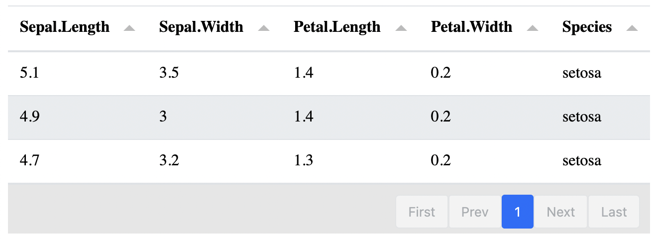
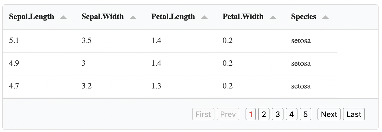
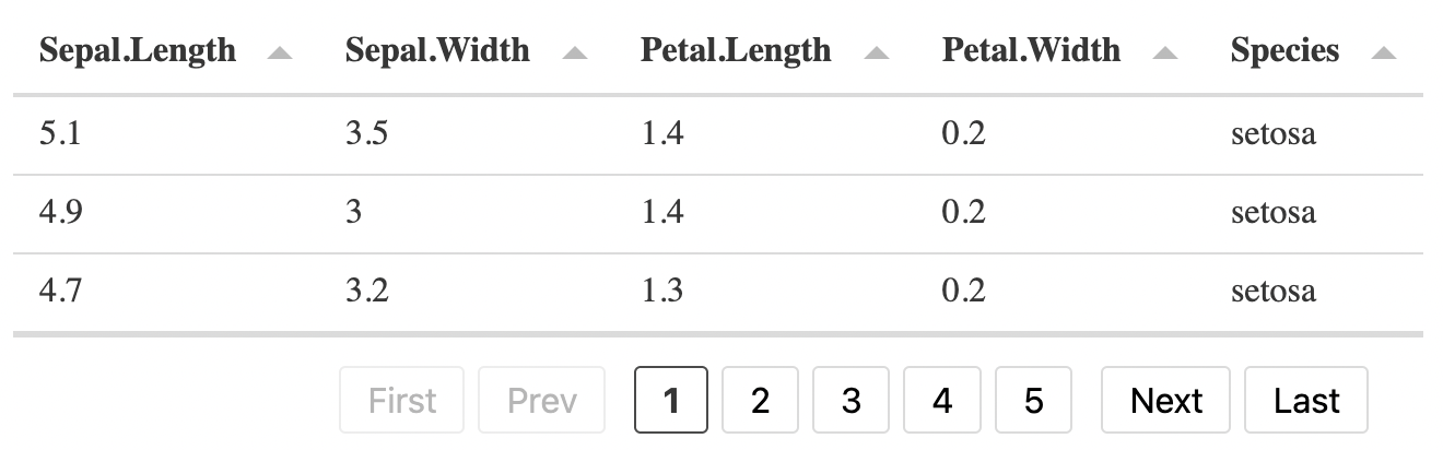
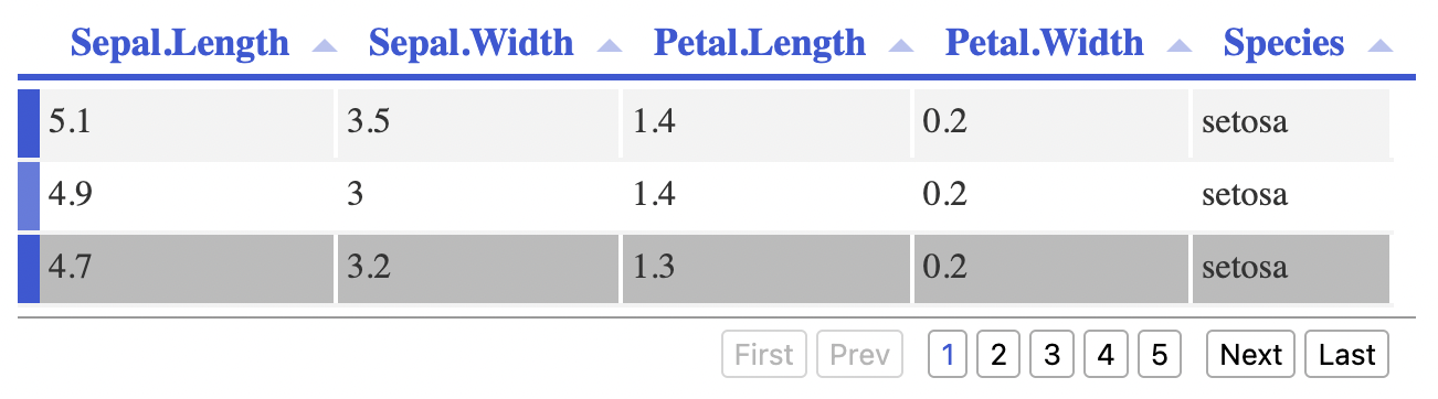
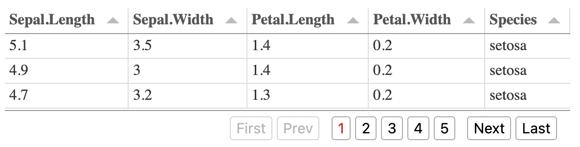
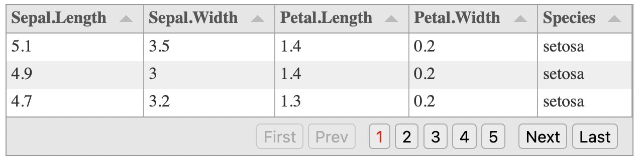
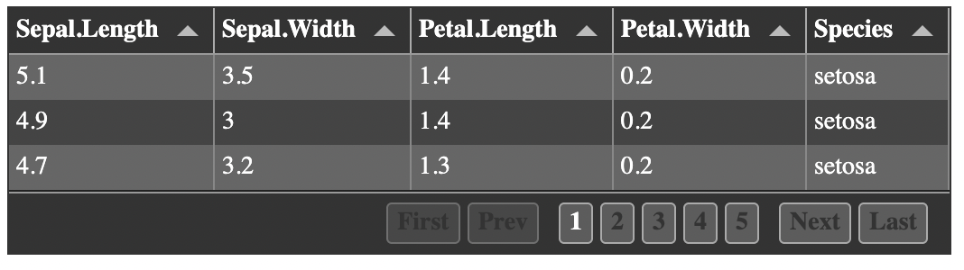
Tabulator ships with multiple complete CSS style sheets. The default in tinytable is Bootstrap 5, but you can customize the appearance using the theme_html() function (when available). Alternatives include "default", "simple", "midnight", "modern", "site", "site_dark", "bootstrap3", "bootstrap4", "bootstrap5", "semanticui", "bulma", and "materialize".

The syntax looks like this:

tt(iris) |> theme_html(tabulator_stylesheet = "semanticui")

Warning

To use a theme, the HTML file must load a style sheet globally in the document. Unfortunately, this means that tinytable cannot apply a Tabulator style sheet to a single table in documents with multiple tables. The style that applies is always the last one loaded in the document.

Here are some screenshots of different stylesheets.