tinytable

Easy, beautiful, and customizable tables in R

tinytable is a small but powerful R package to draw HTML, LaTeX, Word, PDF, Markdown, and Typst tables. The interface is minimalist, but it gives users direct and convenient access to powerful frameworks to create endlessly customizable tables.

Install it from Github:

library(remotes)
install_github("vincentarelbundock/tinytable")

This tutorial introduces the main functions of the package. It is available in two versions:

• PDF
• HTML

Tiny Tables

Load the library and set some global options:

library(tinytable)

options(tinytable_tt_digits = 3)
options(tinytable_theme_placement_latex_float = "H")

Draw a first table:

x <- mtcars[1:4, 1:5]
tt(x)

mpg	cyl	disp	hp	drat
21	6	160	110	3.9
21	6	160	110	3.9
22.8	4	108	93	3.85
21.4	6	258	110	3.08

Width

The width arguments indicating what proportion of the line width the table should cover. This argument accepts a number between 0 and 1 to control the whole table width, or a vector of numeric values between 0 and 1, representing each column.

tt(x, width = 0.5)

mpg	cyl	disp	hp	drat
21	6	160	110	3.9
21	6	160	110	3.9
22.8	4	108	93	3.85
21.4	6	258	110	3.08

tt(x, width = 1)

mpg	cyl	disp	hp	drat
21	6	160	110	3.9
21	6	160	110	3.9
22.8	4	108	93	3.85
21.4	6	258	110	3.08

We can control individual columns by supplying a vector. In that case, the sum of width elements determines the full table width. For example, this table takes 70% of available width, with the first column 3 times as large as the other ones.

tt(x, width = c(.3, .1, .1, .1, .1))

mpg	cyl	disp	hp	drat
21	6	160	110	3.9
21	6	160	110	3.9
22.8	4	108	93	3.85
21.4	6	258	110	3.08

When the sum of the width vector exceeds 1, it is automatically normalized to full-width. This is convenient when we only want to specify column width in relative terms:

tt(x, width = c(3, 2, 1, 1, 1))

mpg	cyl	disp	hp	drat
21	6	160	110	3.9
21	6	160	110	3.9
22.8	4	108	93	3.85
21.4	6	258	110	3.08

When specifying a table width, the text is automatically wrapped to appropriate size:

lorem <- data.frame(
  Lorem = "Sed ut perspiciatis unde omnis iste natus error sit voluptatem accusantium doloremque laudantium, totam rem aperiam, eaque ipsa quae ab illo inventore veritatis et quasi architecto beatae vitae dicta sunt explicabo.",
  Ipsum = " Nemo enim ipsam voluptatem quia voluptas sit aspernatur aut odit aut fugit, sed quia consequuntur magni dolores eos."
)

tt(lorem, width = 3/4)

Lorem	Ipsum
Sed ut perspiciatis unde omnis iste natus error sit voluptatem accusantium doloremque laudantium, totam rem aperiam, eaque ipsa quae ab illo inventore veritatis et quasi architecto beatae vitae dicta sunt explicabo.	Nemo enim ipsam voluptatem quia voluptas sit aspernatur aut odit aut fugit, sed quia consequuntur magni dolores eos.

Footnotes

The notes argument accepts single strings or named lists of strings:

n <- "Fusce id ipsum consequat ante pellentesque iaculis eu a ipsum. Mauris id ex in nulla consectetur aliquam. In nec tempus diam. Aliquam arcu nibh, dapibus id ex vestibulum, feugiat consequat erat. Morbi feugiat dapibus malesuada. Quisque vel ullamcorper felis. Aenean a sem at nisi tempor pretium sit amet quis lacus."

tt(lorem, notes = n, width = 1)

A full-width table with wrapped text in cells and a footnote.

Lorem	Ipsum
Fusce id ipsum consequat ante pellentesque iaculis eu a ipsum. Mauris id ex in nulla consectetur aliquam. In nec tempus diam. Aliquam arcu nibh, dapibus id ex vestibulum, feugiat consequat erat. Morbi feugiat dapibus malesuada. Quisque vel ullamcorper felis. Aenean a sem at nisi tempor pretium sit amet quis lacus.
Sed ut perspiciatis unde omnis iste natus error sit voluptatem accusantium doloremque laudantium, totam rem aperiam, eaque ipsa quae ab illo inventore veritatis et quasi architecto beatae vitae dicta sunt explicabo.	Nemo enim ipsam voluptatem quia voluptas sit aspernatur aut odit aut fugit, sed quia consequuntur magni dolores eos.

When notes is a named list, the names are used as identifiers and displayed as superscripts:

tt(x, notes = list(a = "Blah.", b = "Blah blah."))

mpg	cyl	disp	hp	drat
a Blah.
b Blah blah.
21	6	160	110	3.9
21	6	160	110	3.9
22.8	4	108	93	3.85
21.4	6	258	110	3.08

We can also add markers in individual cells by providing coordinates:

tt(x, notes = list(
    a = list(i = 0:1, j = 1, text = "Blah."),
    b = "Blah blah."
  )
)

mpga	cyl	disp	hp	drat
a Blah.
b Blah blah.
21 a	6	160	110	3.9
21	6	160	110	3.9
22.8	4	108	93	3.85
21.4	6	258	110	3.08

Captions and cross-references

In Quarto, one can specify captions and use cross-references using code like this:

@tbl-blah shows that...

```{r}
#| label: tbl-blah
#| tbl-cap: "Blah blah blah"
library(tinytable)
tt(mtcars[1:4, 1:4])
```

And here is the rendered version of the code chunk above:

Table 1 shows that…

library(tinytable)
tt(mtcars[1:4, 1:4])

Table 1: Blah blah blah

mpg	cyl	disp	hp
21	6	160	110
21	6	160	110
22.8	4	108	93
21.4	6	258	110

For standalone LaTeX tables, you can use the caption argument like so:

tt(x, caption = "Blah blah.\\label{tbl-blah}")

Be aware that this approach may not work well in Quarto or Rmarkdown documents.

Math

To insert LaTeX-style mathematical expressions in a tinytable, we enclose the expression in dollar signs: $...$. The expression will then rendered as a mathematical expression by MathJax (for HTML), LaTeX, or Pandoc. Do not forget to double escape any backslashes.

dat <- data.frame(Math = c(
  "$x^2 + y^2 = z^2$",
  "$\\frac{1}{2}$"
))
tt(dat) |> style_tt(j = 1, align = "c")

Math
$x^2 + y^2 = z^2$
$\frac{1}{2}$

Line breaks and text wrapping

Manual line breaks work sligthly different in LaTeX (PDF) or HTML. This table shows the two strategies. For HTML, we insert a <br> tag. For LaTeX, we wrap the string in curly braces {}, and then insert two (escaped) backslashes: \\\\

d <- data.frame(
  "{Sed ut \\\\ perspiciatis unde}",
  "dicta sunt<br> explicabo. Nemo"
) |> setNames(c("LaTeX line break", "HTML line break"))
tt(d, width = 1)

LaTeX line break	HTML line break
{Sed ut \\ perspiciatis unde}	dicta sunt explicabo. Nemo

Output formats

tinytable can produce tables in HTML, Word, Markdown, LaTeX, Typst, PDF, or PNG format. An appropriate output format for printing is automatically selected based on (1) whether the function is called interactively, (2) is called within RStudio, and (3) the output format of the Rmarkdown or Quarto document, if applicable. Alternatively, users can specify the print format in print() or by setting a global option:

tt(x) |> print("markdown")
tt(x) |> print("html")
tt(x) |> print("latex")

options(tinytable_print_output = "markdown")

With the save_tt() function, users can also save tables directly to PNG (images), PDF or Word documents, and to any of the basic formats. All we need to do is supply a valid file name with the appropriate extension (ex: .png, .html, .pdf, etc.):

tt(x) |> save_tt("path/to/file.png")
tt(x) |> save_tt("path/to/file.pdf")
tt(x) |> save_tt("path/to/file.docx")
tt(x) |> save_tt("path/to/file.html")
tt(x) |> save_tt("path/to/file.tex")
tt(x) |> save_tt("path/to/file.md")

save_tt() can also return a string with the table in it, for further processing in R. In the first case, the table is printed to console with cat(). In the second case, it returns as a single string as an R object.

tt(mtcars[1:10, 1:5]) |>
  group_tt(
    i = list(
      "Hello" = 3,
      "World" = 8),
    j = list(
      "Foo" = 2:3,
      "Bar" = 4:5)) |>
  print("markdown")

+------+-----+------+-----+------+
|      | Foo        | Bar        |
+------+-----+------+-----+------+
| mpg  | cyl | disp | hp  | drat |
+======+=====+======+=====+======+
| 21   | 6   | 160  | 110 | 3.9  |
+------+-----+------+-----+------+
| 21   | 6   | 160  | 110 | 3.9  |
+------+-----+------+-----+------+
| Hello                          |
+------+-----+------+-----+------+
| 22.8 | 4   | 108  | 93  | 3.85 |
+------+-----+------+-----+------+
| 21.4 | 6   | 258  | 110 | 3.08 |
+------+-----+------+-----+------+
| 18.7 | 8   | 360  | 175 | 3.15 |
+------+-----+------+-----+------+
| 18.1 | 6   | 225  | 105 | 2.76 |
+------+-----+------+-----+------+
| 14.3 | 8   | 360  | 245 | 3.21 |
+------+-----+------+-----+------+
| World                          |
+------+-----+------+-----+------+
| 24.4 | 4   | 147  | 62  | 3.69 |
+------+-----+------+-----+------+
| 22.8 | 4   | 141  | 95  | 3.92 |
+------+-----+------+-----+------+
| 19.2 | 6   | 168  | 123 | 3.92 |
+------+-----+------+-----+------+ 

tt(mtcars[1:10, 1:5]) |>
  group_tt(
    i = list(
      "Hello" = 3,
      "World" = 8),
    j = list(
      "Foo" = 2:3,
      "Bar" = 4:5)) |>
  save_tt("markdown")

[1] "+------+-----+------+-----+------+\n|      | Foo        | Bar        |\n+------+-----+------+-----+------+\n| mpg  | cyl | disp | hp  | drat |\n+======+=====+======+=====+======+\n| 21   | 6   | 160  | 110 | 3.9  |\n+------+-----+------+-----+------+\n| 21   | 6   | 160  | 110 | 3.9  |\n+------+-----+------+-----+------+\n| Hello                          |\n+------+-----+------+-----+------+\n| 22.8 | 4   | 108  | 93  | 3.85 |\n+------+-----+------+-----+------+\n| 21.4 | 6   | 258  | 110 | 3.08 |\n+------+-----+------+-----+------+\n| 18.7 | 8   | 360  | 175 | 3.15 |\n+------+-----+------+-----+------+\n| 18.1 | 6   | 225  | 105 | 2.76 |\n+------+-----+------+-----+------+\n| 14.3 | 8   | 360  | 245 | 3.21 |\n+------+-----+------+-----+------+\n| World                          |\n+------+-----+------+-----+------+\n| 24.4 | 4   | 147  | 62  | 3.69 |\n+------+-----+------+-----+------+\n| 22.8 | 4   | 141  | 95  | 3.92 |\n+------+-----+------+-----+------+\n| 19.2 | 6   | 168  | 123 | 3.92 |\n+------+-----+------+-----+------+"

Formatting

Numbers, dates, strings, etc.

The tt() function is minimalist; it’s inteded purpose is simply to draw nice tables. Users who want to format numbers, dates, strings, and other variables in different ways should process their data before supplying it to the tt() table-drawing function. To do so, we can use the format_tt() function supplied by the tinytable.

In a very simple case—such as printing 2 significant digits of all numeric variables—we can use the digits argument of tt():

dat <- data.frame(
     w = c(143002.2092, 201399.181, 100188.3883),
     x = c(1.43402, 201.399, 0.134588),
     y = as.Date(sample(1:1000, 3), origin = "1970-01-01"),
     z = c(TRUE, TRUE, FALSE))

tt(dat, digits = 2)

w	x	y	z
143002	1.43	1971-09-26	True
201399	201.4	1971-01-01	True
100188	0.13	1971-09-17	False

We can get more fine-grained control over formatting by calling format_tt() after tt(), optionally by specifying the columns to format with j:

tt(dat) |> 
  format_tt(
    j = 2:4,
    digits = 1,
    date = "%B %d %Y") |>
  format_tt(
    j = 1,
    digits = 2,
    num_mark_big = " ",
    num_mark_dec = ",",
    num_fmt = "decimal")

w	x	y	z
143 002,21	1.4	September 26 1971	True
201 399,18	201.4	January 01 1971	True
100 188,39	0.1	September 17 1971	False

We can use a regular expression in j to select columns, and the ?sprintf function to format strings, numbers, and to do string interpolation (similar to the glue package, but using Base R):

dat <- data.frame(
     a = c("Burger", "Halloumi", "Tofu", "Beans"),
     b = c(1.43202, 201.399, 0.146188, 0.0031),
     c = c(98938272783457, 7288839482, 29111727, 93945))
tt(dat) |>
  format_tt(j = "a", sprintf = "Food: %s") |>
  format_tt(j = 2, digits = 1) |>
  format_tt(j = "c", digits = 2, num_suffix = TRUE)

a	b	c
Food: Burger	1.432	99T
Food: Halloumi	201.399	7.3B
Food: Tofu	0.146	29M
Food: Beans	0.003	94K

Finally, if you like the format_tt() interface, you can use it directly with numbers, vectors, or data frames:

format_tt(pi, digits = 1)

[1] "3"

format_tt(dat, digits = 1, num_suffix = TRUE)

         a     b   c
1   Burger     1 99T
2 Halloumi   201  7B
3     Tofu   0.1 29M
4    Beans 0.003 94K

Significant digits and decimals

By default, format_tt() formats numbers to ensure that the smallest value in a vector (column) has at least a certain number of significant digits. For example,

k <- data.frame(x = c(0.000123456789, 12.4356789))
tt(k, digits = 2)

x
0.00012
12.43568

We can alter this behavior to ensure to round significant digits on a per-cell basis, using the num_fmt argument in format_tt():

tt(k) |> format_tt(digits = 2, num_fmt = "significant_cell")

x
0.00012
12

The numeric formatting options in format_tt() can also be controlled using global options:

options("tinytable_tt_digits" = 2)
options("tinytable_format_num_fmt" = "significant_cell")
tt(k)

x
0.00012
12

Replacement

Missing values can be replaced by a custom string using the replace argument (default ""):

tab <- data.frame(a = c(NA, 1, 2), b = c(3, NA, 5))

tt(tab)

a	b
NA	3
1	NA
2	5

tt(tab) |> format_tt()

a	b
	3
1
2	5

tt(tab) |> format_tt(replace = "-")

a	b
-	3
1	-
2	5

We can also specify multiple value replacements at once using a named list of vectors:

tmp <- data.frame(x = 1:5, y = c(pi, NA, NaN, -Inf, Inf))
dict <- list("-" = c(NA, NaN), "-∞" = -Inf, "∞" = Inf)
tt(tmp) |> format_tt(replace = dict, digits = 2)

x	y
1	3.1
2	-
3	-
4	-∞
5	∞

Escape special characters

LaTeX and HTML use special characters to indicate strings which should be interpreted rather than displayed as text. For example, including underscores or dollar signs in LaTeX can cause compilation errors in some documents. To display those special characters, we need to substitute or escape them with backslashes, depending on the output format. The escape argument of format_tt() can be used to do this automatically:

dat <- data.frame(
    "LaTeX" = c("Dollars $", "Percent %", "Underscore _"),
    "HTML" = c("<br>", "<sup>4</sup>", "<emph>blah</emph>")
)

tt(dat) |> format_tt(escape = TRUE)

LaTeX	HTML
Dollars $	<br>
Percent %	<sup>4</sup>
Underscore _	<emph>blah</emph>

When applied to a tt() table, format_tt() will determine the type of escaping to do automatically. When applied to a string or vector, we must specify the type of escaping to apply:

format_tt("_ Dollars $", escape = "latex")

[1] "\\_ Dollars \\$"

Markdown

Markdown can be rendered in cells by using the markdown argument of the format_tt() function (note: this requires installing the markdown as an optional dependency).

dat <- data.frame( markdown = c(
  "This is _italic_ text.",
  "This sentence ends with a superscript.^2^")
)

tt(dat) |>
  format_tt(j = 1, markdown = TRUE) |>
  style_tt(j = 1, align = "c")

markdown
This is italic text.
This sentence ends with a superscript.2

Markdown syntax can be particularly useful when formatting URLs in a table:

dat <- data.frame(
  `Package (link)` = c(
    "[`marginaleffects`](https://www.marginaleffects.com/)",
    "[`modelsummary`](https://www.modelsummary.com/)",
    "[`tinytable`](https://vincentarelbundock.github.io/tinytable/)",
    "[`countrycode`](https://vincentarelbundock.github.io/countrycode/)",
    "[`WDI`](https://vincentarelbundock.github.io/WDI/)",
    "[`softbib`](https://vincentarelbundock.github.io/softbib/)",
    "[`tinysnapshot`](https://vincentarelbundock.github.io/tinysnapshot/)",
    "[`altdoc`](https://etiennebacher.github.io/altdoc/)",
    "[`plot2`](https://grantmcdermott.com/plot2/)",
    "[`parameters`](https://easystats.github.io/parameters/)",
    "[`insight`](https://easystats.github.io/insight/)"
  ),
  Purpose = c(
    "Interpreting statistical models",
    "Data and model summaries",
    "Draw beautiful tables easily",
    "Convert country codes and names",
    "Download data from the World Bank",
    "Software bibliographies in R",
    "Snapshots for unit tests using `tinytest`",
    "Create documentation website for R packages",
    "Extension of base R plot functions",
    "Extract from model objects",
    "Extract information from model objects"
  ),
  check.names = FALSE
)

tt(dat) |> format_tt(j = 1, markdown = TRUE)

Vincent sometimes contributes to these R packages.

Package (link)	Purpose
marginaleffects	Interpreting statistical models
modelsummary	Data and model summaries
tinytable	Draw beautiful tables easily
countrycode	Convert country codes and names
WDI	Download data from the World Bank
softbib	Software bibliographies in R
tinysnapshot	Snapshots for unit tests using `tinytest`
altdoc	Create documentation website for R packages
plot2	Extension of base R plot functions
parameters	Extract from model objects
insight	Extract information from model objects

Custom functions

On top of the built-in features of format_tt, a custom formatting function can be specified via the fn argument. The fn argument takes a function that accepts a single vector and returns a string (or something that coerces to a string like a number).

tt(x) |> 
  format_tt(j = "mpg", fn = function(x) paste0(x, " mpg")) |>
  format_tt(j = "drat", fn = \(x) signif(x, 2))

mpg	cyl	disp	hp	drat
21 mpg	6	160	110	3.9
21 mpg	6	160	110	3.9
22.8 mpg	4	108	93	3.8
21.4 mpg	6	258	110	3.1

For example, the scales package which is used internally by ggplot2 provides a bunch of useful tools for formatting (e.g. dates, numbers, percents, logs, currencies, etc.). The label_*() functions can be passed to the fn argument.

Note that we call format_tt(escape = TRUE) at the end of the pipeline because the column names and cells include characters that need to be escaped in LaTeX: _, %, and $. This last call is superfluous in HTML.

thumbdrives <- data.frame(
  date_lookup = as.Date(c("2024-01-15", "2024-01-18", "2024-01-14", "2024-01-16")),
  price = c(18.49, 19.99, 24.99, 24.99),
  price_rank = c(1, 2, 3, 3),
  memory = c(16e9, 12e9, 10e9, 8e9),
  speed_benchmark = c(0.6, 0.73, 0.82, 0.99)
)

tt(thumbdrives) |>
  format_tt(j = 1, fn = scales::label_date("%e %b", locale = "fr")) |>
  format_tt(j = 2, fn = scales::label_currency()) |>
  format_tt(j = 3, fn = scales::label_ordinal()) |> 
  format_tt(j = 4, fn = scales::label_bytes()) |> 
  format_tt(j = 5, fn = scales::label_percent())  |>
  format_tt(escape = TRUE)

date_lookup	price	price_rank	memory	speed_benchmark
2024-01-15	$18.49	1st	16 GB	60%
2024-01-18	$19.99	2nd	12 GB	73%
2024-01-14	$24.99	3rd	10 GB	82%
2024-01-16	$24.99	3rd	8 GB	99%

Style

The main styling function for the tinytable package is style_tt(). Via this function, you can access three main interfaces to customize tables:

1. A general interface to frequently used style choices which works for both HTML and LaTeX (PDF): colors, font style and size, row and column spans, etc. This is accessed through several distinct arguments in the style_tt() function, such as italic, color, etc.
2. A specialized interface which allows users to use the powerful tabularray package to customize LaTeX tables. This is accessed by passing tabularray settings as strings to the tabularray_inner and tabularray_outer arguments of style_tt().
3. A specialized interface which allows users to use the powerful Bootstrap framework to customize HTML tables. This is accessed by passing CSS declarations and rules to the bootstrap_css and bootstrap_css_rule arguments of style_tt().

These functions can be used to customize rows, columns, or individual cells. They control many features, including:

• Text color
• Background color
• Widths
• Heights
• Alignment
• Text Wrapping
• Column and Row Spacing
• Cell Merging
• Multi-row or column spans
• Border Styling
• Font Styling: size, underline, italic, bold, strikethrough, etc.
• Header Customization

The style_*() functions can modify individual cells, or entire columns and rows. The portion of the table that is styled is determined by the i (rows) and j (columns) arguments.

Cells, rows, columns

To style individual cells, we use the style_cell() function. The first two arguments—i and j—identify the cells of interest, by row and column numbers respectively. To style a cell in the 2nd row and 3rd column, we can do:

tt(x) |>
  style_tt(
    i = 2,
    j = 3,
    background = "black",
    color = "white")

mpg	cyl	disp	hp	drat
21.0	6	160	110	3.90
21.0	6	160	110	3.90
22.8	4	108	93	3.85
21.4	6	258	110	3.08

The i and j accept vectors of integers to modify several cells at once:

tt(x) |>
  style_tt(
    i = 2:3,
    j = c(1, 3, 4),
    italic = TRUE,
    color = "orange")

mpg	cyl	disp	hp	drat
21.0	6	160	110	3.90
21.0	6	160	110	3.90
22.8	4	108	93	3.85
21.4	6	258	110	3.08

We can style all cells in a table by omitting both the i and j arguments:

tt(x) |> style_tt(color = "orange")

mpg	cyl	disp	hp	drat
21.0	6	160	110	3.90
21.0	6	160	110	3.90
22.8	4	108	93	3.85
21.4	6	258	110	3.08

We can style entire rows by omitting the j argument:

tt(x) |> style_tt(i = 1:2, color = "orange")

mpg	cyl	disp	hp	drat
21.0	6	160	110	3.90
21.0	6	160	110	3.90
22.8	4	108	93	3.85
21.4	6	258	110	3.08

We can style entire columns by omitting the i argument:

tt(x) |> style_tt(j = c(2, 4), bold = TRUE)

mpg	cyl	disp	hp	drat
21.0	6	160	110	3.90
21.0	6	160	110	3.90
22.8	4	108	93	3.85
21.4	6	258	110	3.08

The j argument accepts integer vectors, character vectors, but also a string with a Perl-style regular expression, which makes it easier to select columns by name:

tt(x) |> style_tt(j = c("mpg", "drat"), color = "orange")

mpg	cyl	disp	hp	drat
21.0	6	160	110	3.90
21.0	6	160	110	3.90
22.8	4	108	93	3.85
21.4	6	258	110	3.08

tt(x) |> style_tt(j = "mpg|drat", color = "orange")

mpg	cyl	disp	hp	drat
21.0	6	160	110	3.90
21.0	6	160	110	3.90
22.8	4	108	93	3.85
21.4	6	258	110	3.08

Here we use a “negative lookahead” to exclude certain columns:

tt(x) |> style_tt(j = "^(?!drat|mpg)", color = "orange")

mpg	cyl	disp	hp	drat
21.0	6	160	110	3.90
21.0	6	160	110	3.90
22.8	4	108	93	3.85
21.4	6	258	110	3.08

Of course, we can also call the style_tt() function several times to apply different styles to different parts of the table:

tt(x) |> 
  style_tt(i = 1, j = 1:2, color = "orange") |>
  style_tt(i = 1, j = 3:4, color = "green")

mpg	cyl	disp	hp	drat
21.0	6	160	110	3.90
21.0	6	160	110	3.90
22.8	4	108	93	3.85
21.4	6	258	110	3.08

Colors

The color and background arguments in the style_tt() function are used for specifying the text color and the background color for cells of a table created by the tt() function. This argument plays a crucial role in enhancing the visual appeal and readability of the table, whether it’s rendered in LaTeX or HTML format. The way we specify colors differs slightly between the two formats:

For HTML Output:

• Hex Codes: You can specify colors using hexadecimal codes, which consist of a # followed by 6 characters (e.g., #CC79A7). This allows for a wide range of colors.
• Keywords: There’s also the option to use color keywords for convenience. The supported keywords are basic color names like black, red, blue, etc.

For LaTeX Output:

• Hexadecimal Codes: Similar to HTML, you can use hexadecimal codes. However, in LaTeX, you need to include these codes as strings (e.g., "#CC79A7").
• Keywords: LaTeX supports a different set of color keywords, which include standard colors like black, red, blue, as well as additional ones like cyan, darkgray, lightgray, etc.
• Color Blending: An advanced feature in LaTeX is color blending, which can be achieved using the xcolor package. You can blend colors by specifying ratios (e.g., white!80!blue or green!20!red).
• Luminance Levels: The ninecolors package in LaTeX offers colors with predefined luminance levels, allowing for more nuanced color choices (e.g., “azure4”, “magenta8”).

Note that the keywords used in LaTeX and HTML are slightly different.

tt(x) |> style_tt(i = 1:4, j = 1, color = "#FF5733")

mpg	cyl	disp	hp	drat
21.0	6	160	110	3.90
21.0	6	160	110	3.90
22.8	4	108	93	3.85
21.4	6	258	110	3.08

Note that when using Hex codes in a LaTeX table, we need extra declarations in the LaTeX preamble. See ?tt for details.

Alignment

To align columns, we use a single character, or a string where each letter represents a column:

dat <- data.frame(
  a = c("a", "aa", "aaa"),
  b = c("b", "bb", "bbb"),
  c = c("c", "cc", "ccc"))

tt(dat) |> style_tt(j = 1:3, align = "c")

a	b	c
a	b	c
aa	bb	cc
aaa	bbb	ccc

tt(dat) |> style_tt(j = 1:3, align = "lcr")

a	b	c
a	b	c
aa	bb	cc
aaa	bbb	ccc

In LaTeX documents (only), we can use decimal-alignment:

z <- data.frame(pi = c(pi * 100, pi * 1000, pi * 10000, pi * 100000))
tt(z) |>
    format_tt(j = 1, digits = 8, num_fmt = "significant_cell") |>
    style_tt(j = 1, align = "d")

pi
314.15927
3141.5927
31415.927
314159.27

Font size

The font size is specified in em units.

tt(x) |> style_tt(j = "mpg|hp|qsec", fontsize = 1.5)

mpg	cyl	disp	hp	drat
21.0	6	160	110	3.90
21.0	6	160	110	3.90
22.8	4	108	93	3.85
21.4	6	258	110	3.08

Spanning cells (merging cells)

Sometimes, it can be useful to make a cell stretch across multiple colums or rows, for example when we want to insert a label. To achieve this, we can use the colspan argument. Here, we make the 2nd cell of the 2nd row stretch across three columns and two rows:

tt(x)|> style_tt(
  i = 2, j = 2,
  colspan = 3,
  rowspan = 2,
  align = "c",
  alignv = "m",
  color = "white",
  background = "black",
  bold = TRUE)

mpg	cyl	disp	hp	drat
21.0	6	160	110	3.90
21.0	6	160	110	3.90
22.8	4	108	93	3.85
21.4	6	258	110	3.08

Here is the original table for comparison:

tt(x)

mpg	cyl	disp	hp	drat
21.0	6	160	110	3.90
21.0	6	160	110	3.90
22.8	4	108	93	3.85
21.4	6	258	110	3.08

Spanning cells can be particularly useful when we want to suppress redundant labels:

tab <- aggregate(mpg ~ cyl + am, FUN = mean, data = mtcars)
tab <- tab[order(tab$cyl, tab$am),]
tab

  cyl am      mpg
1   4  0 22.90000
4   4  1 28.07500
2   6  0 19.12500
5   6  1 20.56667
3   8  0 15.05000
6   8  1 15.40000

tt(tab, digits = 2) |>
  style_tt(i = c(1, 3, 5), j = 1, rowspan = 2, alignv = "t")

cyl	am	mpg
4	0	23
4	1	28
6	0	19
6	1	21
8	0	15
8	1	15

Headers

The header can be omitted from the table by deleting the column names in the x data frame:

k <- x
colnames(k) <- NULL
tt(k)

21.0	6	160	110	3.90
21.0	6	160	110	3.90
22.8	4	108	93	3.85
21.4	6	258	110	3.08

The first is row 0, and higher level headers (ex: column spanning labels) have negative indices like -1. They can be styled as expected:

tt(x) |> style_tt(i = 0, color = "white", background = "black")

mpg	cyl	disp	hp	drat
21.0	6	160	110	3.90
21.0	6	160	110	3.90
22.8	4	108	93	3.85
21.4	6	258	110	3.08

When styling columns without specifying i, the headers are styled in accordance with the rest of the column:

tt(x) |> style_tt(j = 2:3, color = "white", background = "black")

mpg	cyl	disp	hp	drat
21.0	6	160	110	3.90
21.0	6	160	110	3.90
22.8	4	108	93	3.85
21.4	6	258	110	3.08

Conditional styling

We can use the standard which function from Base R to create indices and apply conditional stying on rows. And we can use a regular expression in j to apply conditional styling on columns:

k <- mtcars[1:10, c("mpg", "am", "vs")]

tt(k) |> 
  style_tt(
    i = which(k$am == k$vs),
    background = "teal",
    color = "white")

mpg	am	vs
21.0	1	0
21.0	1	0
22.8	1	1
21.4	0	1
18.7	0	0
18.1	0	1
14.3	0	0
24.4	0	1
22.8	0	1
19.2	0	1

Vectorized styling (heatmaps)

The color, background, and fontsize arguments are vectorized. This allows easy specification of different colors in a single call:

tt(x) |>
  style_tt(
    i = 1:4,
    color = c("red", "blue", "green", "orange"))

mpg	cyl	disp	hp	drat
21.0	6	160	110	3.90
21.0	6	160	110	3.90
22.8	4	108	93	3.85
21.4	6	258	110	3.08

When using a single value for a vectorized argument, it gets applied to all values:

tt(x) |>
  style_tt(
    j = 2:3,
    color = c("orange", "green"),
    background = "black")

mpg	cyl	disp	hp	drat
21.0	6	160	110	3.90
21.0	6	160	110	3.90
22.8	4	108	93	3.85
21.4	6	258	110	3.08

We can also produce more complex heatmap-like tables to illustrate different font sizes in em units:

# font sizes
fs <- seq(.1, 2, length.out = 20)

# headless table
k <- data.frame(matrix(fs, ncol = 5))
colnames(k) <- NULL

# colors
bg <- hcl.colors(20, "Inferno")
fg <- ifelse(as.matrix(k) < 1.7, tail(bg, 1), head(bg, 1))

# table
tt(k, width = .7, theme = "void") |>
  style_tt(j = 1:5, align = "ccccc") |>
  style_tt(
    i = 1:4,
    j = 1:5,
    color = fg,
    background = bg,
    fontsize = fs)

0.1	0.5	0.9	1.3	1.7
0.2	0.6	1.0	1.4	1.8
0.3	0.7	1.1	1.5	1.9
0.4	0.8	1.2	1.6	2.0

Lines (borders)

The style_tt function allows us to customize the borders that surround eacell of a table, as well horizontal and vertical rules. To control these lines, we use the line, line_width, and line_color arguments. Here’s a brief overview of each of these arguments:

• line: This argument specifies where solid lines should be drawn. It is a string that can consist of the following characters:
  • "t": Draw a line at the top of the cell, row, or column.
  • "b": Draw a line at the bottom of the cell, row, or column.
  • "l": Draw a line at the left side of the cell, row, or column.
  • "r": Draw a line at the right side of the cell, row, or column.
  • You can combine these characters to draw lines on multiple sides, such as "tbl" to draw lines at the top, bottom, and left sides of a cell.
• line_width: This argument controls the width of the solid lines in em units (default: 0.1 em). You can adjust this value to make the lines thicker or thinner.
• line_color: Specifies the color of the solid lines. You can use color names, hexadecimal codes, or other color specifications to define the line color.

Here is an example where we draw lines around every border (“t”, “b”, “l”, and “r”) of specified cells.

tt(x, theme = "void") |>
    style_tt(
        i = 0:3,
        j = 1:3,
        line = "tblr",
        line_width = 0.4,
        line_color = "orange")

mpg	cyl	disp	hp	drat
21.0	6	160	110	3.90
21.0	6	160	110	3.90
22.8	4	108	93	3.85
21.4	6	258	110	3.08

And here is an example with horizontal rules:

tt(x, theme = "void") |>
    style_tt(i = 0, line = "t", line_color = "orange", line_width = 0.4) |>
    style_tt(i = 0, line = "b", line_color = "purple", line_width = 0.2) |>
    style_tt(i = 4, line = "b", line_color = "orange", line_width = 0.4)

mpg	cyl	disp	hp	drat
21.0	6	160	110	3.90
21.0	6	160	110	3.90
22.8	4	108	93	3.85
21.4	6	258	110	3.08

dat <- data.frame(1:2, 3:4, 5:6, 7:8)
colnames(dat) <- NULL

tt(dat, theme = "void") |> 
  style_tt(
    line = "tblr", line_color = "white", line_width = 0.5,
    background = "blue", color = "white")

1	3	5	7
2	4	6	8

Cell padding

There is no argument in style_tt() to control the padding of cells. Thankfully, this is easy to control using CSS and tabularray options:

tt(x) |> style_tt(
    i = 1:5,
    bootstrap_css = "padding-right: .2em; padding-top: 2em;",
    tabularray_inner = "rowsep={2em}, colsep = {.2em}"
)

mpg	cyl	disp	hp	drat
21.0	6	160	110	3.90
21.0	6	160	110	3.90
22.8	4	108	93	3.85
21.4	6	258	110	3.08

Markdown and Word

Styling for Markdown and Word tables is more limited than for the other formats. In particular:

• The only supported arguments are: bold, italic, and strikeout.
• Headers inserted by group_tt() cannot be styled using the style_tt() function.

These limitations are due to the fact that there is no markdown syntax for the other options (ex: colors and background), and that we create Word documents by converting a markdown table to .docx via the Pandoc software.

One workaround is to style the group headers directly in their definition by using markdown syntax:

mtcars[1:4, 1:4] |>
  tt() |>
  group_tt(i = list("*Hello*" = 1, "__World__" = 3)) |>
  print("markdown")

+------+-----+------+-----+
| mpg  | cyl | disp | hp  |
+======+=====+======+=====+
| *Hello*                 |
+------+-----+------+-----+
| 21.0 | 6   | 160  | 110 |
+------+-----+------+-----+
| 21.0 | 6   | 160  | 110 |
+------+-----+------+-----+
| __World__               |
+------+-----+------+-----+
| 22.8 | 4   | 108  |  93 |
+------+-----+------+-----+
| 21.4 | 6   | 258  | 110 |
+------+-----+------+-----+ 

Plots and images

The plot_tt() function can embed images and plots in a tinytable. We can insert images by specifying their paths and positions (i/j).

Inserting images in tables

To insert images in a table, we use the plot_tt() function. The path_img values must be relative to the main document saved by save_tt() or to the Quarto (or Rmarkdown) document in which the code is executed.

dat <- data.frame(
  Species = c("Spider", "Squirrel"),
  Image = ""
)

img <- c(
  "../figures/spider.png",
  "../figures/squirrel.png"
)

tt(dat) |>
  plot_tt(j = 2, images = img, height = 3)

Species	Image
Spider
Squirrel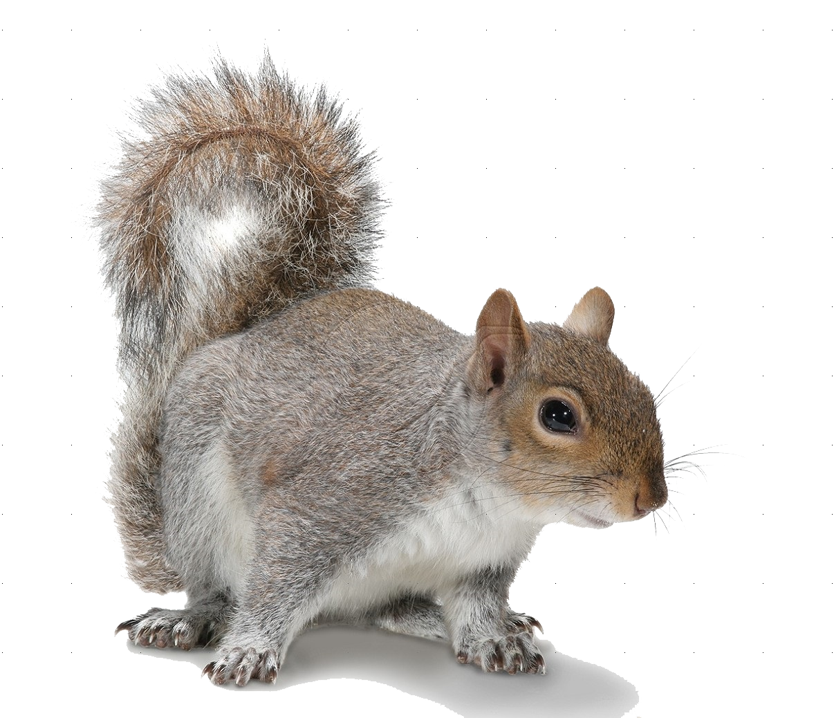

In HTML tables, it is possible to insert tables directly from a web address, but not in LaTeX.

dat <- data.frame("R" = "")
img <- "https://cran.r-project.org/Rlogo.svg"
tt(dat) |>
  plot_tt(i = 1, j = 1, images = img, height = 7) |>
  style_tt(j = 1, align = "c")

R

Inline plots

We can draw inline plots three ways, with

1. Built-in templates for histograms, density plots, and bar plots
2. Custom plots using base R plots.
3. Custom plots using ggplot2.

To draw custom plots, one simply has to define a custom function, whose structure we illustrate below.

Built-in plots

There are several types of inline plots available by default. For example,

plot_data <- list(mtcars$mpg, mtcars$hp, mtcars$qsec)

dat <- data.frame(
  Variables = c("mpg", "hp", "qsec"), 
  Histogram = "",
  Density = "",
  Bar = "",
  Line = ""
)

# random data for sparklines
lines <- lapply(1:3, \(x) data.frame(x = 1:10, y = rnorm(10)))

tt(dat) |>
  plot_tt(j = 2, fun = "histogram", data = plot_data) |>
  plot_tt(j = 3, fun = "density", data = plot_data, color = "darkgreen") |>
  plot_tt(j = 4, fun = "bar", data = list(2, 3, 6), color = "orange") |>
  plot_tt(j = 5, fun = "line", data = lines, color = "blue") |>
  style_tt(j = 2:5, align = "c")

Variables	Histogram	Density	Bar	Line
mpg
hp
qsec

Custom plots: Base R

Important: Custom functions must have ... as an argument.

To create a custom inline plot using Base R plotting functions, we create a function that returns another function. tinytable will then call that second function internally to generate the plot.

This is easier than it sounds! For example:

f <- function(d, ...) {
  function() hist(d, axes = FALSE, ann = FALSE, col = "lightblue")
}

plot_data <- list(mtcars$mpg, mtcars$hp, mtcars$qsec)

dat <- data.frame(Variables = c("mpg", "hp", "qsec"), Histogram = "")

tt(dat) |>
  plot_tt(j = 2, fun = f, data = plot_data)

Variables	Histogram
mpg
hp
qsec

Custom plots: ggplot2

Important: Custom functions must have ... as an argument.

To create a custom inline plot using ggplot2, we create a function that returns a ggplot object:

library(ggplot2)

f <- function(d, color = "black", ...) {
  d <- data.frame(x = d)
  ggplot(d, aes(x = x)) + 
    geom_histogram(bins = 30, color = color, fill = color) +
    scale_x_continuous(expand=c(0,0)) +
    scale_y_continuous(expand=c(0,0)) +
    theme_void()
}

plot_data <- list(mtcars$mpg, mtcars$hp, mtcars$qsec)

tt(dat) |>
  plot_tt(j = 2, fun = f, data = plot_data, color = "pink")

Variables	Histogram
mpg
hp
qsec

We can insert arbitrarily complex plots by customizing the ggplot2 call:

penguins <- read.csv(
  "https://vincentarelbundock.github.io/Rdatasets/csv/palmerpenguins/penguins.csv",
  na.strings = "") |> na.omit()

# split data by species
dat <- split(penguins, penguins$species)
body <- lapply(dat, \(x) x$body_mass_g)
flip <- lapply(dat, \(x) x$flipper_length_mm)

# create nearly empty table
tab <- data.frame(
  "Species" = names(dat),
  "Body Mass" = "",
  "Flipper Length" = "",
  "Body vs. Flipper" = "",
  check.names = FALSE
)

# custom ggplot2 function to create inline plot
f <- function(d, ...) {
  ggplot(d, aes(x = flipper_length_mm, y = body_mass_g, color = sex)) +
    geom_point(size = .2) +
    scale_x_continuous(expand=c(0,0)) +
    scale_y_continuous(expand=c(0,0)) +
    scale_color_manual(values = c("#E69F00", "#56B4E9")) +
    theme_void() +
    theme(legend.position = "none")
}

# `tinytable` calls
tt(tab) |>
  plot_tt(j = 2, fun = "histogram", data = body, height = 2) |>
  plot_tt(j = 3, fun = "density", data = flip, height = 2) |>
  plot_tt(j = 4, fun = f, data = dat, height = 2) |>
  style_tt(j = 2:4, align = "c") 

Species	Body Mass	Flipper Length	Body vs. Flipper
Adelie
Chinstrap
Gentoo

Fontawesome

We can use the fontawesome package to include fancy icons in HTML tables:

library(fontawesome)
tmp <- mtcars[1:4, 1:4]
tmp[1, 1] <- paste(fa("r-project"), "for statistics")
tt(tmp)

mpg	cyl	disp	hp
for statistics	6	160	110
21	6	160	110
22.8	4	108	93
21.4	6	258	110

Groups and labels

The group_tt() function can label groups of rows (i) or columns (j).

Rows

The i argument accepts a named list of integers. The numbers identify the positions where row group labels are to be inserted. The names includes the text that should be inserted:

dat <- mtcars[1:9, 1:8]

tt(dat) |>
  group_tt(i = list(
    "I like (fake) hamburgers" = 3,
    "She prefers halloumi" = 4,
    "They love tofu" = 7))

mpg	cyl	disp	hp	drat	wt	qsec	vs
21.0	6	160.0	110	3.90	2.620	16.46	0
21.0	6	160.0	110	3.90	2.875	17.02	0
22.8	4	108.0	93	3.85	2.320	18.61	1
21.4	6	258.0	110	3.08	3.215	19.44	1
18.7	8	360.0	175	3.15	3.440	17.02	0
18.1	6	225.0	105	2.76	3.460	20.22	1
14.3	8	360.0	245	3.21	3.570	15.84	0
24.4	4	146.7	62	3.69	3.190	20.00	1
22.8	4	140.8	95	3.92	3.150	22.90	1

We can style group rows in the same way as regular rows:

tt(dat) |> 
  group_tt(
    i = list(
      "I like (fake) hamburgers" = 3,
      "She prefers halloumi" = 4,
      "They love tofu" = 7)) |>
  style_tt(
    i = c(3, 5, 9),
    align = "c",
    color = "white",
    background = "gray",
    bold = TRUE)

mpg	cyl	disp	hp	drat	wt	qsec	vs
21.0	6	160.0	110	3.90	2.620	16.46	0
21.0	6	160.0	110	3.90	2.875	17.02	0
22.8	4	108.0	93	3.85	2.320	18.61	1
21.4	6	258.0	110	3.08	3.215	19.44	1
18.7	8	360.0	175	3.15	3.440	17.02	0
18.1	6	225.0	105	2.76	3.460	20.22	1
14.3	8	360.0	245	3.21	3.570	15.84	0
24.4	4	146.7	62	3.69	3.190	20.00	1
22.8	4	140.8	95	3.92	3.150	22.90	1

Columns

The syntax for column groups is very similar, but we use the j argument instead. The named list specifies the labels to appear in column-spanning labels, and the values must be a vector of consecutive and non-overlapping integers that indicate which columns are associated to which labels:

tt(dat) |> 
  group_tt(
    j = list(
      "Hamburgers" = 1:3,
      "Halloumi" = 4:5,
      "Tofu" = 7))

Hamburgers			Halloumi			Tofu
mpg	cyl	disp	hp	drat	wt	qsec	vs
21.0	6	160.0	110	3.90	2.620	16.46	0
21.0	6	160.0	110	3.90	2.875	17.02	0
22.8	4	108.0	93	3.85	2.320	18.61	1
21.4	6	258.0	110	3.08	3.215	19.44	1
18.7	8	360.0	175	3.15	3.440	17.02	0
18.1	6	225.0	105	2.76	3.460	20.22	1
14.3	8	360.0	245	3.21	3.570	15.84	0
24.4	4	146.7	62	3.69	3.190	20.00	1
22.8	4	140.8	95	3.92	3.150	22.90	1

Here is a table with both row and column headers, as well as some styling:

dat <- mtcars[1:9, 1:8]
tt(dat) |> 
  group_tt(
    i = list("I like (fake) hamburgers" = 3,
             "She prefers halloumi" = 4,
             "They love tofu" = 7),
    j = list("Hamburgers" = 1:3,
             "Halloumi" = 4:5,
             "Tofu" = 7)) |>
  style_tt(
    i = c(3, 5, 9),
    align = "c",
    background = "teal",
    color = "white") |>
  style_tt(i = -1, color = "teal")

Hamburgers			Halloumi			Tofu
mpg	cyl	disp	hp	drat	wt	qsec	vs
21.0	6	160.0	110	3.90	2.620	16.46	0
21.0	6	160.0	110	3.90	2.875	17.02	0
22.8	4	108.0	93	3.85	2.320	18.61	1
21.4	6	258.0	110	3.08	3.215	19.44	1
18.7	8	360.0	175	3.15	3.440	17.02	0
18.1	6	225.0	105	2.76	3.460	20.22	1
14.3	8	360.0	245	3.21	3.570	15.84	0
24.4	4	146.7	62	3.69	3.190	20.00	1
22.8	4	140.8	95	3.92	3.150	22.90	1

We can also stack several extra headers on top of one another:

tt(x) |>
  group_tt(j = list("Foo" = 2:3, "Bar" = 5)) |>
  group_tt(j = list("Hello" = 1:2, "World" = 4:5))

Hello			World
	Foo			Bar
mpg	cyl	disp	hp	drat
21.0	6	160	110	3.90
21.0	6	160	110	3.90
22.8	4	108	93	3.85
21.4	6	258	110	3.08

Themes

tinytable offers a very flexible theming framwork, which includes a few basic visual looks, as well as other functions to apply collections of transformations to tinytable objects in a repeatable way. These themes can be applied by supplying a string or function to the theme argument in tt(). Alternatively, users can call the theme_tt() function.

The main difference between theme_tt() and the other options in package, is that whereas style_tt() and format_tt() aim to be output agnostic, theme_tt() supplies transformations that can be output-specific, and which can have their own sets of distinct arguments. See below for a few examples.

Visual themes

To begin, let’s explore a few of the basic looks supplied by themes:

tt(x, theme = "striped")

mpg	cyl	disp	hp	drat
21.0	6	160	110	3.90
21.0	6	160	110	3.90
22.8	4	108	93	3.85
21.4	6	258	110	3.08

tt(x) |> theme_tt("striped")

mpg	cyl	disp	hp	drat
21.0	6	160	110	3.90
21.0	6	160	110	3.90
22.8	4	108	93	3.85
21.4	6	258	110	3.08

tt(x, theme = "grid")

mpg	cyl	disp	hp	drat
21.0	6	160	110	3.90
21.0	6	160	110	3.90
22.8	4	108	93	3.85
21.4	6	258	110	3.08

tt(x, theme = "bootstrap")

mpg	cyl	disp	hp	drat
21.0	6	160	110	3.90
21.0	6	160	110	3.90
22.8	4	108	93	3.85
21.4	6	258	110	3.08

Custom themes

Users can also define their own themes to apply consistent visual tweaks to tables. For example, this defines a themeing function and sets a global option to apply it to all tables consistently:

theme_vincent <- function(x, ...) {
  out <- x |> 
    style_tt(color = "teal") |>
    theme_tt("placement")
  out@caption <- "Always use the same caption."
  return(out)
}

options(tinytable_tt_theme = theme_vincent)

tt(mtcars[1:2, 1:2])

Always use the same caption.

mpg	cyl
21	6
21	6

tt(mtcars[1:3, 1:3])

Always use the same caption.

mpg	cyl	disp
21.0	6	160
21.0	6	160
22.8	4	108

options(tinytable_tt_theme = NULL)

Tabular

The tabular theme is designed to provide a more “raw” table, without a floating table environment in LaTeX, and without CSS or Javascript in HTML.

tt(x) |> theme_tt("tabular") |> print("latex")

\begin{tblr}[         %% tabularray outer open
]                     %% tabularray outer close
{                     %% tabularray inner open
colspec={Q[]Q[]Q[]Q[]Q[]},
}                     %% tabularray inner close
\toprule
mpg & cyl & disp & hp & drat \\ \midrule %% TinyTableHeader
21.0 & 6 & 160 & 110 & 3.90 \\
21.0 & 6 & 160 & 110 & 3.90 \\
22.8 & 4 & 108 &  93 & 3.85 \\
21.4 & 6 & 258 & 110 & 3.08 \\
\bottomrule
\end{tblr} 

Resize

LaTeX only.

Placement

LaTeX only.

Multipage

LaTeX only.

Combination and exploration

Tables can be explored, modified, and combined using many of the usual base R functions:

a <- tt(mtcars[1:2, 1:2])
a

mpg	cyl
21	6
21	6

dim(a)

[1] 2 2

ncol(a)

[1] 2

nrow(a)

[1] 2

colnames(a)

[1] "mpg" "cyl"

Rename columns:

colnames(a) <- c("a", "b")
a

a	b
21	6
21	6

Tables can be combined with the usual rbind() function:

a <- tt(mtcars[1:3, 1:2], caption = "Combine two tiny tables.")
b <- tt(mtcars[4:5, 8:10]) 

rbind(a, b)

Combine two tiny tables.

mpg	cyl	vs	am	gear
21.0	6	NA	NA	NA
21.0	6	NA	NA	NA
22.8	4	NA	NA	NA
NA	NA	vs	am	gear
NA	NA	1	0	3
NA	NA	0	0	3

rbind(a, b) |> format_tt(replace = "")

Combine two tiny tables.

mpg	cyl	vs	am	gear
21.0	6
21.0	6
22.8	4
		vs	am	gear
		1	0	3
		0	0	3

The rbind2() S4 method is slightly more flexible than rbind(), as it supports arguments headers and use.names.

Omit y header:

rbind2(a, b, headers = FALSE)

Combine two tiny tables.

mpg	cyl	vs	am	gear
21.0	6	NA	NA	NA
21.0	6	NA	NA	NA
22.8	4	NA	NA	NA
NA	NA	1	0	3
NA	NA	0	0	3

Bind tables by position rather than column names:

rbind2(a, b, use_names = FALSE)

Combine two tiny tables.

mpg	cyl	gear
21.0	6	NA
21.0	6	NA
22.8	4	NA
vs	am	gear
1	0	3
0	0	3

HTML customization

Bootstrap classes

The Bootstrap framework provides a number of built-in themes to style tables, using “classes.” To use them, we call style_tt() with the bootstrap_class argument. A list of available Bootstrap classes can be found here: https://getbootstrap.com/docs/5.3/content/tables/

For example, to produce a “bordered” table, we use the table-bordered class:

tt(x) |> style_tt(bootstrap_class = "table table-bordered")

mpg	cyl	disp	hp	drat
21.0	6	160	110	3.90
21.0	6	160	110	3.90
22.8	4	108	93	3.85
21.4	6	258	110	3.08

We can also combine several Bootstrap classes. Here, we get a table with the “hover” feature:

tt(x) |> style_tt(
  bootstrap_class = "table table-hover")

mpg	cyl	disp	hp	drat
21.0	6	160	110	3.90
21.0	6	160	110	3.90
22.8	4	108	93	3.85
21.4	6	258	110	3.08

CSS declarations

The style_tt() function allows us to declare CSS properties and values for individual cells, columns, or rows of a table. For example, if we want to make the first column bold, we could do:

tt(x) |>
  style_tt(j = 1, bootstrap_css = "font-weight: bold; color: red;")

mpg	cyl	disp	hp	drat
21.0	6	160	110	3.90
21.0	6	160	110	3.90
22.8	4	108	93	3.85
21.4	6	258	110	3.08

CSS rules

For more extensive customization, we can use complete CSS rules. In this example, we define several rules that apply to a new class called mytable. Then, we use the theme argument of the tt() function to ensure that our tiny table is of class mytable. Finally, we call style_bootstrap() to apply the rules with the bootstrap_css_rule argument.

css_rule <- "
.mytable {
  background: linear-gradient(45deg, #EA8D8D, #A890FE);
  width: 600px;
  border-collapse: collapse;
  overflow: hidden;
  box-shadow: 0 0 20px rgba(0,0,0,0.1);
}

.mytable th,
.mytable td {
  padding: 5px;
  background-color: rgba(255,255,255,0.2);
  color: #fff;
}

.mytable tbody tr:hover {
  background-color: rgba(255,255,255,0.3);
}

.mytable tbody td:hover:before {
  content: '';
  position: absolute;
  left: 0;
  right: 0;
  top: -9999px;
  bottom: -9999px;
  background-color: rgba(255,255,255,0.2);
  z-index: -1;
}
"

tt(x, width = 2/3) |> 
  style_tt(
    j = 1:5,
    align = "ccccc",
    bootstrap_class = "table mytable",
    bootstrap_css_rule = css_rule)

mpg	cyl	disp	hp	drat
21.0	6	160	110	3.90
21.0	6	160	110	3.90
22.8	4	108	93	3.85
21.4	6	258	110	3.08

And here’s another example:

css <- "
.squirreltable {
  background-size: cover;
  background-position: center;
  background-image: url('https://user-images.githubusercontent.com/987057/82732352-b9aabf00-9cda-11ea-92a6-26750cf097d0.png');
  --bs-table-bg: transparent;
}
"

tt(mtcars[1:10, 1:8]) |>
  style_tt(
    bootstrap_class = "table table-borderless squirreltable", 
    bootstrap_css_rule = css)

mpg	cyl	disp	hp	drat	wt	qsec	vs
21.0	6	160.0	110	3.90	2.620	16.46	0
21.0	6	160.0	110	3.90	2.875	17.02	0
22.8	4	108.0	93	3.85	2.320	18.61	1
21.4	6	258.0	110	3.08	3.215	19.44	1
18.7	8	360.0	175	3.15	3.440	17.02	0
18.1	6	225.0	105	2.76	3.460	20.22	1
14.3	8	360.0	245	3.21	3.570	15.84	0
24.4	4	146.7	62	3.69	3.190	20.00	1
22.8	4	140.8	95	3.92	3.150	22.90	1
19.2	6	167.6	123	3.92	3.440	18.30	1

LaTeX / PDF customization

The LaTeX / PDF customization options described in this section are not available for HTML documents. Please refer to the PDF documentation hosted on the website to read this part of the tutorial.

Preamble

Introduction to tabularray

tabularray keys

Shiny

tinytable is a great complement to Shiny for displaying HTML tables in a web app. The styling in a tinytable is applied by JavaScript functions and CSS. Thus, to ensure that this styling is preserved in a Shiny app, one strategy is to bake the entire page, save it in a temporary file, and load it using the includeHTML function from the shiny package. This approach is illustrated in this minimal example:

library("shiny")
library("tinytable")

fn <- paste(tempfile(), ".html")
tab <- tt(mtcars[1:5, 1:4]) |> 
  style_tt(i = 0:5, color = "orange", background = "black") |> 
  save_tt(fn) 

shinyApp(
  ui = fluidPage(
    fluidRow(column(12, h1("This is test of tinytable"), 
                    shiny::includeHTML(fn)))), 
  server = function(input, output) { 
  }
)