Getting started

To begin, load the modelsummary package and download data from the Rdatasets archive:

library(modelsummary)
library(tinytable)

url <- 'https://vincentarelbundock.github.io/Rdatasets/csv/HistData/Guerry.csv'
dat <- read.csv(url) 
dat$Small <- dat$Pop1831 > median(dat$Pop1831)
dat <- dat[, 
  c("Donations", "Literacy", "Commerce", "Crime_pers", "Crime_prop", "Clergy", "Small")
]

Data Summaries

Quick overview of the data:

datasummary_skim(dat)

Warning: The `replace_na` argument was renamed `replace`.

tinytable_7cnux598ooxqo5huuvtt

	Unique	Missing Pct.	Mean	SD	Min	Median	Max
Donations	85	0	7075.5	5834.6	1246.0	5020.0	37015.0
Literacy	50	0	39.3	17.4	12.0	38.0	74.0
Commerce	84	0	42.8	25.0	1.0	42.5	86.0
Crime_pers	85	0	19754.4	7504.7	2199.0	18748.5	37014.0
Crime_prop	86	0	7843.1	3051.4	1368.0	7595.0	20235.0
Clergy	85	0	43.4	25.0	1.0	43.5	86.0
Small	N	%
FALSE	43	50.0
TRUE	43	50.0

Balance table (aka “Table 1”) with differences in means by subgroups:

datasummary_balance(~Small, dat)

tinytable_4i9oc35rwp6r3qkhxiw4

	FALSE (N=43)		TRUE (N=43)
	Mean	Std. Dev.	Mean	Std. Dev.	Diff. in Means	Std. Error
Donations	7258.5	6194.1	6892.6	5519.0	-365.9	1265.2
Literacy	37.9	19.1	40.6	15.6	2.7	3.8
Commerce	42.7	24.6	43.0	25.7	0.3	5.4
Crime_pers	18040.6	7638.4	21468.2	7044.3	3427.7	1584.6
Crime_prop	8422.5	3406.7	7263.7	2559.3	-1158.8	649.8
Clergy	39.1	26.7	47.7	22.7	8.6	5.3

Correlation table:

datasummary_correlation(dat)

tinytable_ffokqp12nqsbdx0mrx04

	Donations	Literacy	Commerce	Crime_pers	Crime_prop	Clergy
Donations	1	.	.	.	.	.
Literacy	-.13	1	.	.	.	.
Commerce	.30	-.58	1	.	.	.
Crime_pers	-.04	-.04	.05	1	.	.
Crime_prop	-.13	-.37	.41	.27	1	.
Clergy	.09	-.17	-.12	.26	-.07	1

Two variables and two statistics, nested in subgroups:

datasummary(Literacy + Commerce ~ Small * (mean + sd), dat)

tinytable_qr0uq4itl4e4s7csh8kz

	FALSE		TRUE
	mean	sd	mean	sd
Literacy	37.88	19.08	40.63	15.57
Commerce	42.65	24.59	42.95	25.75

Model Summaries

Estimate a linear model and display the results:

mod <- lm(Donations ~ Crime_prop, data = dat)

modelsummary(mod)

tinytable_y0v09xaqt6b4ey6dqj7c

	(1)
(Intercept)	9065.287
	(1738.926)
Crime_prop	-0.254
	(0.207)
Num.Obs.	86
R2	0.018
R2 Adj.	0.006
AIC	1739.0
BIC	1746.4
Log.Lik.	-866.516
F	1.505
RMSE	5749.29

Now estimate five regression models, display the results side-by-side, and use the group_tt() function from the tinytable package to add column labels:

library(tinytable)

models <- list(
    "I" = lm(Donations ~ Literacy + Clergy, data = dat),
    "II" = lm(Crime_pers ~ Literacy + Clergy, data = dat),
    "III" = lm(Crime_prop ~ Literacy + Clergy, data = dat),
    "IV" = glm(Crime_pers ~ Literacy + Commerce, family = poisson, data = dat),
    "V" = glm(Donations ~ Literacy + Commerce, family = poisson, data = dat)
)

modelsummary(models, stars = TRUE, gof_omit = "IC|Adj|F|RMSE|Log") |>
    group_tt(j = list("Linear" = 2:4, "Poisson" = 5:6))

tinytable_qx4fzgvntf5e6r2llsg1

	Linear			Poisson
	I	II	III	IV	V
+ p
(Intercept)	7948.667***	16259.384***	11243.544***	9.876***	8.241***
	(2078.276)	(2611.140)	(1011.240)	(0.003)	(0.006)
Literacy	-39.121	3.680	-68.507***	0.000***	0.003***
	(37.052)	(46.552)	(18.029)	(0.000)	(0.000)
Clergy	15.257	77.148*	-16.376
	(25.735)	(32.334)	(12.522)
Commerce				0.001***	0.011***
				(0.000)	(0.000)
Num.Obs.	86	86	86	86	86
R2	0.020	0.065	0.152

Now, save it to a Microsoft Word document:

modelsummary(models, output = "table.docx")

And draw a coefficient plot:

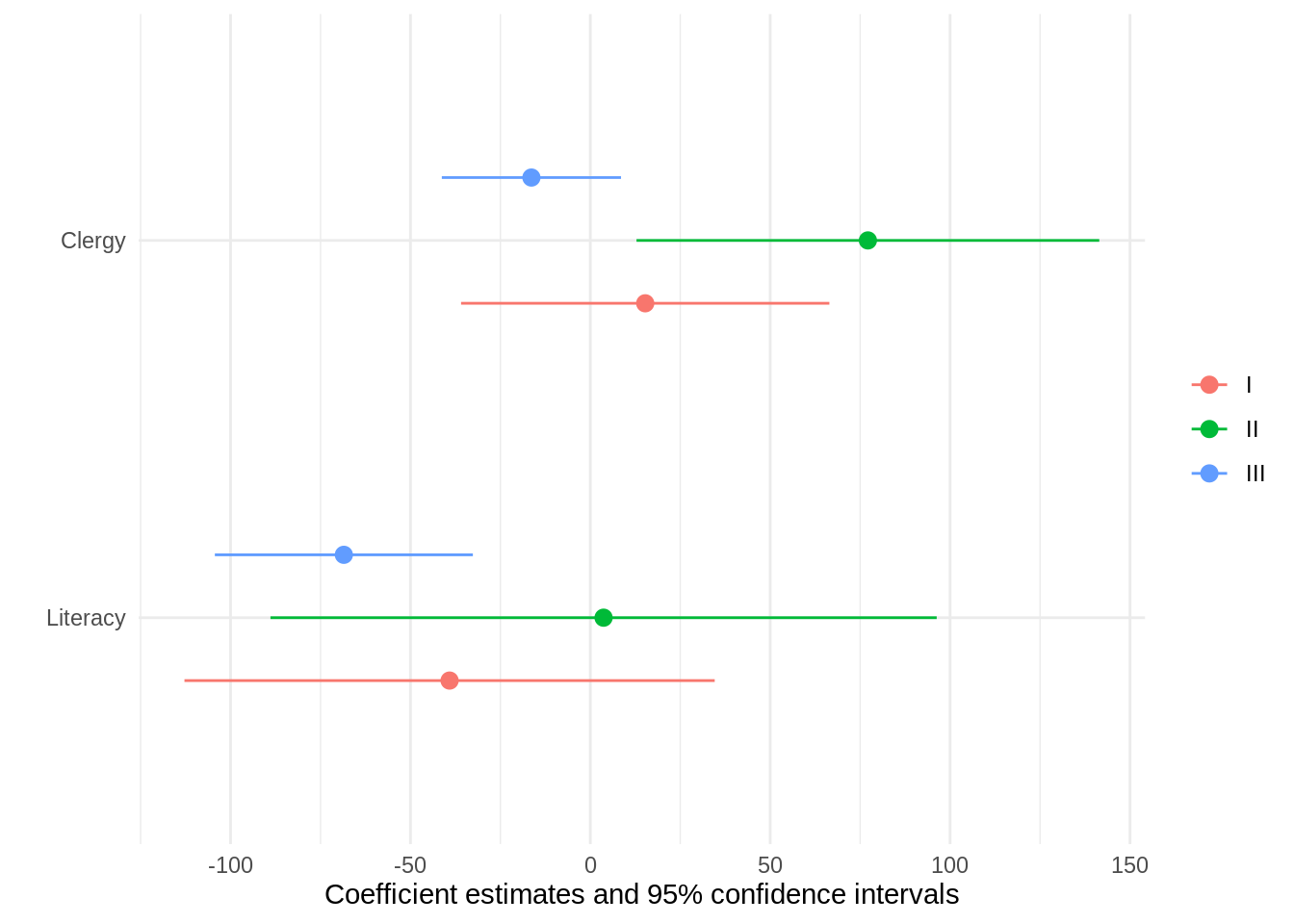
ols <- models[1:3]
modelplot(ols, coef_omit = "Intercept")