Data Summaries

datasummary is a function from the modelsummary package. It allows us to create data summaries, frequency tables, crosstabs, correlation tables, balance tables (aka “Table 1”), and more. It has many benefits:

Easy to use.
Extremely flexible.
Many output formats: HTML, LaTeX, Microsoft Word and Powerpoint, Text/Markdown, PDF, RTF, or Image files.
Embed tables in Rmarkdown or knitr dynamic documents.
Customize the appearance of tables with the tinytable, gt, kableExtra or flextable packages. The possibilities are endless!

This tutorial will show how to draw tables like these (and more!):

datasummary is built around the fantastic tables package for R. It is a thin “wrapper” which adds convenience functions and arguments; a user-interface consistent with modelsummary; cleaner html output; and the ability to export tables to more formats, including gt tables, flextable objects, and Microsoft Word documents.

datasummary is a general-purpose table-making tool. It allows us to build (nearly) any summary table we want by using simple 2-sided formulae. For example, in the expression x + y ~ mean + sd, the left-hand side of the formula identifies the variables or statistics to display as rows, and the right-hand side defines the columns. Below, we will see how variables and statistics can be “nested” with the * operator to produce tables like the ones above.

In addition to datasummary, the modelsummary package includes a “family” of companion functions named datasummary_*. These functions facilitate the production of standard, commonly used tables. This family currently includes:

datasummary(): Flexible function to create custom tables using 2-sided formulae.
datasummary_balance(): Group characteristics (e.g., control vs. treatment)
datasummary_correlation(): Table of correlations.
datasummary_skim(): Quick summary of a dataset.
datasummary_df(): Create a table from any dataframe.
datasummary_crosstab(): Cross tabulations of categorical variables.

In the next three sections, we illustrate how to use datasummary_balance, datasummary_correlation, datasummary_skim, and datasummary_crosstab. Then, we dive into datasummary itself to highlight its ease and flexibility.

`datasummary_skim`

The first datasummary companion function is called datasummary_skim. It was heavily inspired by one of my favorite data exploration tools for R: the skimr package. The goal of this function is to give us a quick look at the data.

To illustrate, we download data from the cool new palmerpenguins package by Alison Presmanes Hill and Allison Horst. These data were collected at the Palmer Station in Antarctica by Gorman, Williams & Fraser (2014), and they include 3 categorical variables and 4 numeric variables.

library(modelsummary)
library(tidyverse)

url <- 'https://vincentarelbundock.github.io/Rdatasets/csv/palmerpenguins/penguins.csv'
penguins <- read.csv(url, na.strings = "")

To summarize the numeric variables in the dataset, we type:

datasummary_skim(penguins)

Warning: The `replace_na` argument was renamed `replace`.

tinytable_t6zzfv2022zywy5xg5sf

	Unique	Missing Pct.	Mean	SD	Min	Median	Max
rownames	344	0	172.5	99.4	1.0	172.5	344.0
bill_length_mm	165	1	43.9	5.5	32.1	44.5	59.6
bill_depth_mm	81	1	17.2	2.0	13.1	17.3	21.5
flipper_length_mm	56	1	200.9	14.1	172.0	197.0	231.0
body_mass_g	95	1	4201.8	802.0	2700.0	4050.0	6300.0
year	3	0	2008.0	0.8	2007.0	2008.0	2009.0
		N	%
species	Adelie	152	44.2
	Chinstrap	68	19.8
	Gentoo	124	36.0
island	Biscoe	168	48.8
	Dream	124	36.0
	Torgersen	52	15.1
sex	female	165	48.0
	male	168	48.8
	NA	11	3.2

To summarize the categorical variables in the dataset, we type:

datasummary_skim(penguins, type = "categorical")

tinytable_lj1lx591q4ucqjtx2lci

		N	%
species	Adelie	152	44.2
	Chinstrap	68	19.8
	Gentoo	124	36.0
island	Biscoe	168	48.8
	Dream	124	36.0
	Torgersen	52	15.1
sex	female	165	48.0
	male	168	48.8
	NA	11	3.2

`datasummary_balance`

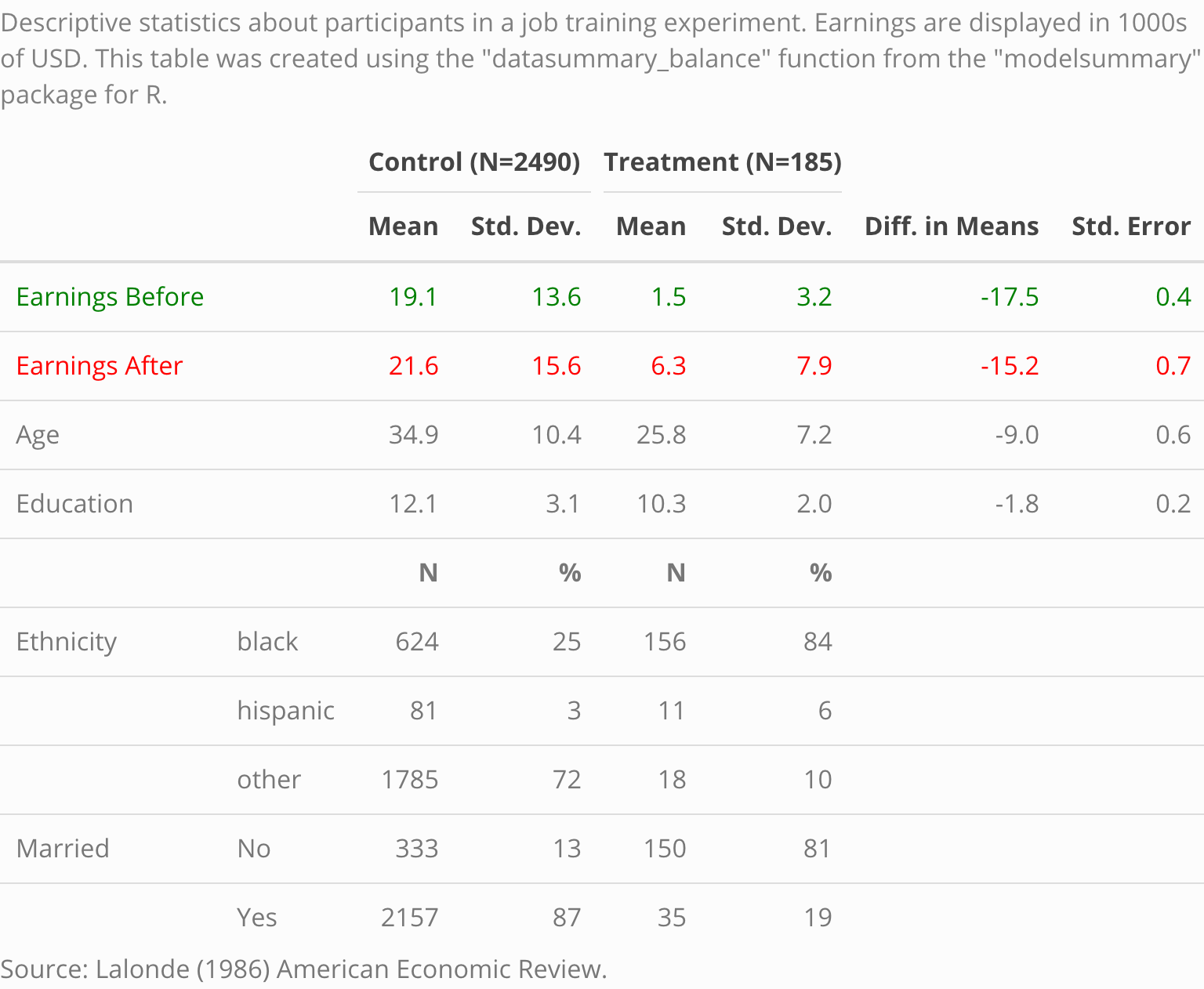
The expressions “balance table” or “Table 1” refer to a type of table which is often printed in the opening pages of a scientific peer-reviewed article. Typically, this table includes basic descriptive statistics about different subsets of the study population. For instance, analysts may want to compare the socio-demographic characteristics of members of the “control” and “treatment” groups in a randomized control trial, or the flipper lengths of male and female penguins. In addition, balance tables often include difference in means tests.

To illustrate how to build a balance table using the datasummary_balance function, we download data about a job training experiment studies in Lalonde (1986). Then, we clean up the data by renaming and recoding a few variables.

# Download and read data
training <- 'https://vincentarelbundock.github.io/Rdatasets/csv/Ecdat/Treatment.csv'
training <- read.csv(training, na.strings = "")

# Rename and recode variables
training <- training %>%
            mutate(`Earnings Before` = re75 / 1000,
                   `Earnings After` = re78 / 1000,
                   Treatment = ifelse(treat == TRUE, 'Treatment', 'Control'),
                   Married = ifelse(married == TRUE, 'Yes', 'No')) %>%
            select(`Earnings Before`,
                   `Earnings After`,
                   Treatment,
                   Ethnicity = ethn,
                   Age = age,
                   Education = educ,
                   Married)

Now, we execute the datasummary_balance function. If the estimatr package is installed, datasummary_balance will calculate the difference in means and test statistics.

caption <- 'Descriptive statistics about participants in a job training experiment. The earnings are displayed in 1000s of USD. This table was created using the "datasummary" function from the "modelsummary" package for R.'
reference <- 'Source: Lalonde (1986) American Economic Review.'

library(modelsummary)
datasummary_balance(~Treatment,
                    data = training,
                    title = caption,
                    notes = reference)

Note that if the dataset includes columns called “blocks”, “clusters”, or “weights”, this information will automatically be taken into consideration by estimatr when calculating the difference in means and the associated statistics.

Users can also use the ~ 1 formula to indicate that they want to summarize all the data instead of splitting the analysis across subgroups:

datasummary_balance(~ 1, data = training)

tinytable_goehyid6xttllb686nhy

		Mean	Std. Dev.
Earnings Before		17.9	13.9
Earnings After		20.5	15.6
Age		34.2	10.5
Education		12.0	3.1
		N	Pct.
Treatment	Control	2490	93.1
	Treatment	185	6.9
Ethnicity	black	780	29.2
	hispanic	92	3.4
	other	1803	67.4
Married	No	483	18.1
	Yes	2192	81.9

`datasummary_correlation`

The datasummary_correlation accepts a dataframe or tibble, it identifies all the numeric variables, and calculates the correlation between each of those variables:

datasummary_correlation(mtcars)

tinytable_1ats7kfxe9c1o6rl828y

	mpg	cyl	disp	hp	drat	wt	qsec	vs	am	gear	carb
mpg	1	.	.	.	.	.	.	.	.	.	.
cyl	-.85	1	.	.	.	.	.	.	.	.	.
disp	-.85	.90	1	.	.	.	.	.	.	.	.
hp	-.78	.83	.79	1	.	.	.	.	.	.	.
drat	.68	-.70	-.71	-.45	1	.	.	.	.	.	.
wt	-.87	.78	.89	.66	-.71	1	.	.	.	.	.
qsec	.42	-.59	-.43	-.71	.09	-.17	1	.	.	.	.
vs	.66	-.81	-.71	-.72	.44	-.55	.74	1	.	.	.
am	.60	-.52	-.59	-.24	.71	-.69	-.23	.17	1	.	.
gear	.48	-.49	-.56	-.13	.70	-.58	-.21	.21	.79	1	.
carb	-.55	.53	.39	.75	-.09	.43	-.66	-.57	.06	.27	1

The values displayed in this table are equivalent to those obtained by calling: cor(x, use='pairwise.complete.obs').

The datasummary_correlation function has a methods argument. The default value is "pearson", but it also accepts other values like "spearman". In addition, method can accept any function which takes a data frame and returns a matrix. For example, we can create a custom function to display information from the correlation package. This allows us to include significance stars even if the stars argument is not supported by default in datasummary_correlation():

library(correlation)

fun <- function(x) {
  out <- correlation(mtcars) |>
    summary() |>
    format(2) |> 
    as.matrix()
  row.names(out) <- out[, 1]
  out <- out[, 2:ncol(out)]
  return(out)
}

datasummary_correlation(mtcars, method = fun)

tinytable_oqnzae3e3czpb9mwzn4g

	carb	gear	am	vs	qsec	wt	drat	hp	disp	cyl
mpg	-.55*	.48	.60**	.66**	.42	-.87***	.68***	-.78***	-.85***	-.85***
cyl	.53*	-.49	-.52*	-.81***	-.59*	.78***	-.70***	.83***	.90***
disp	.39	-.56*	-.59*	-.71***	-.43	.89***	-.71***	.79***
hp	.75***	-.13	-.24	-.72***	-.71***	.66**	-.45
drat	-.09	.70***	.71***	.44	.09	-.71***
wt	.43	-.58*	-.69***	-.55*	-.17
qsec	-.66**	-.21	-.23	.74***
vs	-.57*	.21	.17
am	.06	.79***
gear	.27

`datasummary_crosstab`

A cross tabulation is often useful to explore the association between two categorical variables.

library(modelsummary)
url <- 'https://vincentarelbundock.github.io/Rdatasets/csv/palmerpenguins/penguins.csv'
penguins <- read.csv(url, na.strings = "")

datasummary_crosstab(species ~ sex, data = penguins)

tinytable_p9bm9vqfkh3f6hy9i014

species		female	male	All
Adelie	N	73	73	152
	% row	48.0	48.0	100.0
Chinstrap	N	34	34	68
	% row	50.0	50.0	100.0
Gentoo	N	58	61	124
	% row	46.8	49.2	100.0
All	N	165	168	344
	% row	48.0	48.8	100.0

You can create multi-level crosstabs by specifying interactions using the * operator:

datasummary_crosstab(species ~ sex * island, data = penguins)

tinytable_cd68da9q80hirpxub3rl

		female			male
species		Biscoe	Dream	Torgersen	Biscoe	Dream	Torgersen	All
Adelie	N	22	27	24	22	28	23	152
	% row	14.5	17.8	15.8	14.5	18.4	15.1	100.0
Chinstrap	N	0	34	0	0	34	0	68
	% row	0.0	50.0	0.0	0.0	50.0	0.0	100.0
Gentoo	N	58	0	0	61	0	0	124
	% row	46.8	0.0	0.0	49.2	0.0	0.0	100.0
All	N	80	61	24	83	62	23	344
	% row	23.3	17.7	7.0	24.1	18.0	6.7	100.0

By default, the cell counts and row percentages are shown for each cell, and both row and column totals are calculated. To show cell percentages or column percentages, or to drop row and column totals, adjust the statistic argument. This argument accepts a formula that follows the datasummary “language”. To understand exactly how it works, you may find it useful to skip to the datasummary tutorial in the next section. Example:

datasummary_crosstab(species ~ sex,
                     statistic = 1 ~ Percent("col"),
                     data = penguins)

tinytable_ijo6e376zf85ijh2b69h

species		female	male
Adelie	% col	44.2	43.5
Chinstrap	% col	20.6	20.2
Gentoo	% col	35.2	36.3
All	% col	100.0	100.0

See ?datasummary_crosstab for more details.

`datasummary`

datasummary tables are specified using a 2-sided formula, divided by a tilde ~. The left-hand side describes the rows; the right-hand side describes the columns. To illustrate how this works, we will again be using the palmerpenguins dataset:

To display the flipper_length_mm variable as a row and the mean as a column, we type:

datasummary(flipper_length_mm ~ Mean,
            data = penguins)

tinytable_zyq8g0ugk49xb85nu053

	Mean
flipper_length_mm	200.92

To flip rows and columns, we flip the left and right-hand sides of the formula:

datasummary(Mean ~ flipper_length_mm,
            data = penguins)

tinytable_0vkipjr8ywm424rresng

	flipper_length_mm
Mean	200.92

Custom summary functions

The Mean function is a shortcut supplied by modelsummary, and it is equivalent to mean(x,na.rm=TRUE). Since the flipper_length_mm variable includes missing observation, using the mean formula (with default na.rm=FALSE) would produce a missing/empty cell:

datasummary(flipper_length_mm ~ mean,
            data = penguins)

tinytable_z98l8hpbp1zd4p62fdrc

	mean
flipper_length_mm

modelsummary supplies these functions: Mean, SD, Min, Max, Median, P0, P25, P50, P75, P100, Histogram, and a few more (see the package documentation).

Users are also free to create and use their own custom summaries. Any R function which takes a vector and produces a single value is acceptable. For example, the Range functions return a numerical value, and the MinMax returns a string:

Range <- function(x) max(x, na.rm = TRUE) - min(x, na.rm = TRUE)

datasummary(flipper_length_mm ~ Range,
            data = penguins)

tinytable_44iqb9oyufupkekc1qfd

	Range
flipper_length_mm	59.00

MinMax <- function(x) paste0('[', min(x, na.rm = TRUE), ', ', max(x, na.rm = TRUE), ']')

datasummary(flipper_length_mm ~ MinMax,
            data = penguins)

tinytable_2ifkyydss2xdbbikhkww

	MinMax
flipper_length_mm	[172, 231]

Concatenating with `+`

To include more rows and columns, we use the + sign:

datasummary(flipper_length_mm + body_mass_g ~ Mean + SD,
            data = penguins)

tinytable_mn8m9xg70iic9wpnupi2

	Mean	SD
flipper_length_mm	200.92	14.06
body_mass_g	4201.75	801.95

Sometimes, it can be cumbersome to list all variables separated by + signs. The All() function is a useful shortcut:

datasummary(All(penguins) ~ Mean + SD,
            data = penguins)

tinytable_9b3eqvvn2nrikxkl7n8c

	Mean	SD
rownames	172.50	99.45
bill_length_mm	43.92	5.46
bill_depth_mm	17.15	1.97
flipper_length_mm	200.92	14.06
body_mass_g	4201.75	801.95
year	2008.03	0.82

By default, All selects all numeric variables. This behavior can be changed by modifying the function’s arguments. See ?All for details.

Nesting with `*`

datasummary can nest variables and statistics inside categorical variables using the * symbol. When applying the the * operator to factor, character, or logical variables, columns or rows will automatically be nested. For instance, if we want to display separate means for each value of the variable sex, we use mean * sex:

datasummary(flipper_length_mm + body_mass_g ~ mean * sex,
            data = penguins)

tinytable_d47qn2vhr3myiap8hlxl

	female	male
flipper_length_mm	197.36	204.51
body_mass_g	3862.27	4545.68

We can use parentheses to nest several terms inside one another, using a call of this form: x * (y + z). Here is an example with nested columns:

datasummary(body_mass_g ~ sex * (mean + sd),
            data = penguins)

tinytable_p684z7dwd7h9e3lzr78u

	female		male
	mean	sd	mean	sd
body_mass_g	3862.27	666.17	4545.68	787.63

Here is an example with nested rows:

datasummary(sex * (body_mass_g + flipper_length_mm) ~ mean + sd,
            data = penguins)

tinytable_etgfhp11t2png6680min

sex		mean	sd
female	body_mass_g	3862.27	666.17
	flipper_length_mm	197.36	12.50
male	body_mass_g	4545.68	787.63
	flipper_length_mm	204.51	14.55

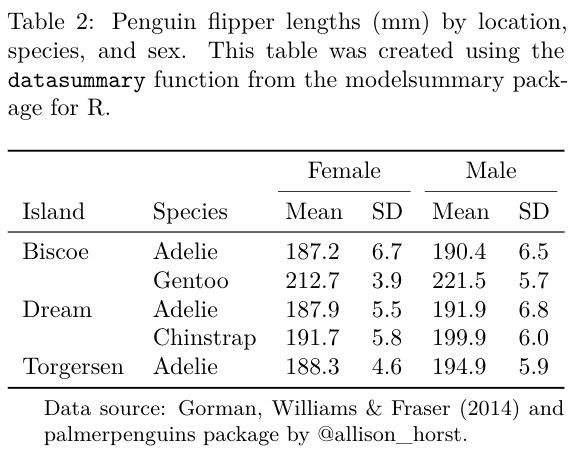
The order in which terms enter the formula determines the order in which labels are displayed. For example, this shows island above sex:

datasummary(flipper_length_mm + body_mass_g ~ mean * island * sex,
            data = penguins)

tinytable_va7r09azrwohv9jwf3k2

	Biscoe		Dream		Torgersen
	female	male	female	male	female	male
flipper_length_mm	205.69	213.29	190.02	196.31	188.29	194.91
body_mass_g	4319.38	5104.52	3446.31	3987.10	3395.83	4034.78

This shows sex above island values:

datasummary(flipper_length_mm + body_mass_g ~ mean * sex * island,
            data = penguins)

tinytable_mta0jdcmbqthuyky0hqt

	female			male
	Biscoe	Dream	Torgersen	Biscoe	Dream	Torgersen
flipper_length_mm	205.69	190.02	188.29	213.29	196.31	194.91
body_mass_g	4319.38	3446.31	3395.83	5104.52	3987.10	4034.78

By default, datasummary omits column headers with a single value/label across all columns, except for the header that sits just above the data. If the header we want to see is not displayed, we may want to reorder the terms of the formula. To show all headers, set sparse_header=FALSE:

datasummary(flipper_length_mm + body_mass_g ~ mean * sex * island,
            data = penguins,
            sparse_header = FALSE)

tinytable_ku7fve2yec86bg8vvn7u

	female			male
	Biscoe	Dream	Torgersen	Biscoe	Dream	Torgersen
flipper_length_mm	205.69	190.02	188.29	213.29	196.31	194.91
body_mass_g	4319.38	3446.31	3395.83	5104.52	3987.10	4034.78

When using sparse_header=FALSE, it is often useful to insert Heading() * in the table formula, in order to rename or omit some of the labels manually. Type ?tables::Heading for details and examples.

Renaming with `=`

Personally, I prefer to rename variables and values before drawing my tables, using backticks when variable names include whitespace. For example,

tmp <- penguins %>%
       select(`Flipper length (mm)` = flipper_length_mm,
              `Body mass (g)` = body_mass_g)

datasummary(`Flipper length (mm)` + `Body mass (g)` ~ Mean + SD,
            data = tmp)

tinytable_0foz4cd6fsw6wlomwz1j

	Mean	SD
Flipper length (mm)	200.92	14.06
Body mass (g)	4201.75	801.95

However, thanks to the tables package, datasummary offers two additional mechanisms to rename. First, we can wrap a term in parentheses and use the equal = sign: (NewName=OldName):

datasummary((`Flipper length (mm)` = flipper_length_mm) + (`Body mass (g)` = body_mass_g) ~
            island * ((Avg. = Mean) + (Std.Dev. = SD)),
            data = penguins)

tinytable_u7kf6ggra125w080lfky

	Biscoe		Dream		Torgersen
	Avg.	Std.Dev.	Avg.	Std.Dev.	Avg.	Std.Dev.
Flipper length (mm)	209.71	14.14	193.07	7.51	191.20	6.23
Body mass (g)	4716.02	782.86	3712.90	416.64	3706.37	445.11

Second, we can use the Heading() function:

datasummary(Heading("Flipper length (mm)") * flipper_length_mm + Heading("Body mass (g)") * body_mass_g ~ island * (Mean + SD),
            data = penguins)

tinytable_yib054i7npnuhuxy3uc0

	Biscoe		Dream		Torgersen
	Mean	SD	Mean	SD	Mean	SD
Flipper length (mm)	209.71	14.14	193.07	7.51	191.20	6.23
Body mass (g)	4716.02	782.86	3712.90	416.64	3706.37	445.11

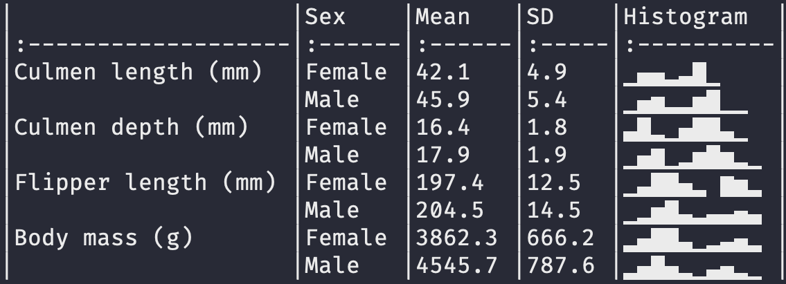
The Heading function also has a nearData argument which can be useful in cases where some rows are nested but others are not. Compare the last row of these two tables:

datasummary(sex * (flipper_length_mm + bill_length_mm) + Heading("Body mass (g)") * body_mass_g ~ Mean + SD,
            data = penguins)

tinytable_t5sy22ruze6suwwluc15

sex		Mean	SD
female	flipper_length_mm	197.36	12.50
	bill_length_mm	42.10	4.90
male	flipper_length_mm	204.51	14.55
	bill_length_mm	45.85	5.37
	Body mass (g)	4201.75	801.95

datasummary(sex * (flipper_length_mm + bill_length_mm) + Heading("Body mass (g)", nearData=FALSE) * body_mass_g ~ Mean + SD,
            data = penguins)

tinytable_5n1wdyt4nn7mfexgeriw

sex		Mean	SD
female	flipper_length_mm	197.36	12.50
	bill_length_mm	42.10	4.90
male	flipper_length_mm	204.51	14.55
	bill_length_mm	45.85	5.37
Body mass (g)		4201.75	801.95

Counts and Percentages

The tables package allows datasummary to use neat tricks to produce frequency tables:

Add a N to the right-hand side of the equation.
Add Percent() to the right-hand side to calculate the percentage of observations in each cell.
Add 1 to the left-hand side to include a row with the total number of observations:

datasummary(species * sex + 1 ~ N + Percent(),
            data = penguins)

tinytable_fbqkupaay9kk43y70rxu

species	sex	N	Percent
Adelie	female	73	21.22
	male	73	21.22
Chinstrap	female	34	9.88
	male	34	9.88
Gentoo	female	58	16.86
	male	61	17.73
	All	344	100.00

Note that the Percent() function accepts a denom argument to determine if percentages should be calculated row or column-wise, or if they should take into account all cells.

Weighted percentages

The Percent() pseudo-function also accepts a fn argument, which must be a function which accepts two vectors: x is the values in the current cell, and y is all the values in the whole dataset. The default fn is:

datasummary(species * sex + 1 ~ N + Percent(fn = function(x, y) 100 * length(x) / length(y)),
            data = penguins)

tinytable_328vy4ndy9idg89k8nlg

species	sex	N	Percent
Adelie	female	73	21.22
	male	73	21.22
Chinstrap	female	34	9.88
	male	34	9.88
Gentoo	female	58	16.86
	male	61	17.73
	All	344	100.00

The code above takes the number of elements in the cell length(x) and divides it by the number of total elements length(y).

Now, let’s say we want to display percentages weighted by one of the variables of the dataset. This can often be useful with survey weights, for example. Here, we use an arbitrary column of weights called flipper_length_mm:

wtpct <- function(x, y) sum(x, na.rm = TRUE) / sum(y, na.rm = TRUE) * 100
datasummary(species * sex + 1 ~ N + flipper_length_mm * Percent(fn = wtpct),
            data = penguins)

tinytable_u6d7l3uln73uop08cu45

species	sex	N	Percent
Adelie	female	73	19.95
	male	73	20.44
Chinstrap	female	34	9.49
	male	34	9.89
Gentoo	female	58	17.95
	male	61	19.67
	All	344	100.00

In each cell we now have the sum of weights in that cell, divided by the total sum of weights in the column.

Custom percentages

Here is another simple illustration of Percent function mechanism in action, where we combine counts and percentages in a simple nice label:

dat <- mtcars
dat$cyl <- as.factor(dat$cyl)

fn <- function(x, y) {
    out <- sprintf(
        "%s (%.1f%%)",
        length(x),
        length(x) / length(y) * 100)
}
datasummary(
    cyl ~ Percent(fn = fn),
    data = dat)

tinytable_rzjnv5tovk81vserwj7b

cyl	Percent
4	11 (34.4%)
6	7 (21.9%)
8	14 (43.8%)

`Factor`

The * nesting operator that we used above works automatically for factor, character, and logical variables. Sometimes, it is convenient to use it with other types of variables, such as binary numeric variables. In that case, we can wrap the variable name inside a call to Factor(). This allows us to treat a variable as factor, without having to modify it in the original data. For example, in the mtcars data, there is a binary numeric variable call am. We nest statistics within categories of am by typing:

datasummary(mpg + hp ~ Factor(am) * (mean + sd),
            data = mtcars)

tinytable_qi4xw0mh6npoza9yweh7

	0		1
	mean	sd	mean	sd
mpg	17.15	3.83	24.39	6.17
hp	160.26	53.91	126.85	84.06

`Arguments`: `na.rm=TRUE`

We can pass any argument to the summary function by including a call to Arguments(). For instance, there are missing values in the flipper_length_mm variable of the penguins dataset. Therefore, the standard mean function will produce no result, because its default argument is na.rm=FALSE. We can change that by calling:

datasummary(flipper_length_mm ~ mean + mean*Arguments(na.rm=TRUE),
            data = penguins)

tinytable_7lplnchpoi78h883car7

	mean	mean
flipper_length_mm		200.92

Notice that there is an empty cell (NA) under the normal mean function, but that the mean call with Arguments(na.rm=TRUE) produced a numeric result.

We can pass the same arguments to multiple functions using the parentheses:

datasummary(flipper_length_mm ~ (mean + sd) * Arguments(na.rm=TRUE),
            data = penguins)

tinytable_xp71zhgx1ol9rk980d6b

	mean	sd
flipper_length_mm	200.92	14.06

Note that the shortcut functions that modelsummary supplies use na.rm=TRUE by default, so we can use them directly without arguments, even when there are missing values:

datasummary(flipper_length_mm ~ Mean + Var + P75 + Range,
            data = penguins)

tinytable_23zkrk7228zase24rcc4

	Mean	Var	P75	Range
flipper_length_mm	200.92	197.73	213.00	59.00

`Arguments`: Weighted Mean

You can use the Arguments mechanism to do various things, such as calculating weighted means:

newdata <- data.frame(
  x = rnorm(20),
  w = rnorm(20),
  y = rnorm(20))

datasummary(x + y ~ weighted.mean * Arguments(w = w),
            data = newdata)

tinytable_pqhr3ghydm7xvf236c08

	weighted.mean
x	1.42
y	-0.75

Which produces the same results as:

weighted.mean(newdata$x, newdata$w)

[1] 1.422057

weighted.mean(newdata$y, newdata$w)

[1] -0.7466463

But different results from:

mean(newdata$x)

[1] -0.2021528

mean(newdata$y)

[1] 0.07847319

Logical subsets

Cool stuff is possible with logical subsets:

datasummary((bill_length_mm > 44.5) + (bill_length_mm <= 44.5) ~ Mean * flipper_length_mm,
            data = penguins)

tinytable_gtx9o7om8zjexgcl9brs


bill_length_mm > 44.5	209.68
bill_length_mm	192.45

See the tables package documentation for more details and examples.

Missing values

At least 3 distinct issues can arise related to missing values.

Functions and `na.rm`

An empty cell can appear in the table when a statistical function returns NA instead of a numeric value. In those cases, you should:

Make sure that your statistical function (e.g., mean or sd) uses na.rm=TRUE by default
Use the Arguments strategy to set na.rm=TRUE (see the Arguments section of this vignette).
Use a convenience function supplied by modelsummary, where na.rm is TRUE by default: Mean, SD, P25, etc.

Empty crosstab cells

An empty cell can appear in the table when a crosstab is deeply nested, and there are no observations for a given combination of covariates. In those cases, you can use the * DropEmpty pseudo-function. See the “Empty cells” section of this vignette for examples.

datasummary(island * species * body_mass_g ~ sex * (Mean + SD),
            data = penguins)

tinytable_bbw7yhn44fbw5qzyewud

			female		male
island	species		Mean	SD	Mean	SD
Biscoe	Adelie	body_mass_g	3369.32	343.47	4050.00	355.57
	Chinstrap	body_mass_g
	Gentoo	body_mass_g	4679.74	281.58	5484.84	313.16
Dream	Adelie	body_mass_g	3344.44	212.06	4045.54	330.55
	Chinstrap	body_mass_g	3527.21	285.33	3938.97	362.14
	Gentoo	body_mass_g
Torgersen	Adelie	body_mass_g	3395.83	259.14	4034.78	372.47
	Chinstrap	body_mass_g
	Gentoo	body_mass_g

datasummary(island * species * body_mass_g ~ sex * (Mean + SD) * DropEmpty(),
            data = penguins)

tinytable_uu7ngtvf8b85e07ikq52

			female		male
island	species		Mean	SD	Mean	SD
Biscoe	Adelie	body_mass_g	3369.32	343.47	4050.00	355.57
	Gentoo	body_mass_g	4679.74	281.58	5484.84	313.16
Dream	Adelie	body_mass_g	3344.44	212.06	4045.54	330.55
	Chinstrap	body_mass_g	3527.21	285.33	3938.97	362.14
Torgersen	Adelie	body_mass_g	3395.83	259.14	4034.78	372.47

Percent()

By default, the Percent() function computes the share of each category with respect to the whole data, including missing observations, but we can work around this with some trickery:jig

dat <- data.frame(z = c(0,0,1,0,NA,0,1))

prop.table(table(dat$z))


        0         1 
0.6666667 0.3333333

datasummary(Factor(z) ~ N + Percent(), data = dat)

tinytable_fl8dp690cjyqi68nw87u

z	N	Percent
0	4	57.14
1	2	28.57

To count percentages without missing values, we can exploit the fact that Percent() accepts a denom argument which can be a logical vector:

datasummary(Factor(z) ~ N + Percent(denom = !is.na(dat$z)), data = dat)

tinytable_3gexp9sq6ht5daub6cja

z	N	Percent
0	4	66.67
1	2	33.33

Add rows

new_rows <- data.frame('Does',
                       2,
                       'plus',
                       2,
                       'equals',
                       5,
                       '?')
datasummary(flipper_length_mm + body_mass_g ~ species * (Mean + SD),
            data = penguins,
            add_rows = new_rows)

tinytable_h6wddykjyu3w0011cspr

	Adelie		Chinstrap		Gentoo
	Mean	SD	Mean	SD	Mean	SD
flipper_length_mm	189.95	6.54	195.82	7.13	217.19	6.48
body_mass_g	3700.66	458.57	3733.09	384.34	5076.02	504.12
Does	2.00	plus	2.00	equals	5.00	?

Add columns

new_cols <- data.frame('New Stat' = runif(2))
datasummary(flipper_length_mm + body_mass_g ~ species * (Mean + SD),
            data = penguins,
            add_columns = new_cols)

tinytable_onbjvp2gd1cb0it034mv

	Adelie		Chinstrap		Gentoo
	Mean	SD	Mean	SD	Mean	SD	New.Stat
flipper_length_mm	189.95	6.54	195.82	7.13	217.19	6.48	0.97
body_mass_g	3700.66	458.57	3733.09	384.34	5076.02	504.12	0.20

Output formats

All functions in the datasummary_* family accept the same output argument. Tables can be saved to several file formats:

f <- flipper_length_mm ~ island * (mean + sd)
datasummary(f, data = penguins, output = 'table.html')
datasummary(f, data = penguins, output = 'table.tex')
datasummary(f, data = penguins, output = 'table.docx')
datasummary(f, data = penguins, output = 'table.pptx')
datasummary(f, data = penguins, output = 'table.md')
datasummary(f, data = penguins, output = 'table.rtf')
datasummary(f, data = penguins, output = 'table.jpg')
datasummary(f, data = penguins, output = 'table.png')

They can be returned in human-readable data.frames, markdown, html, or LaTeX code to the console:

datasummary(f, data = penguins, output = 'data.frame')
datasummary(f, data = penguins, output = 'markdown')
datasummary(f, data = penguins, output = 'html')
datasummary(f, data = penguins, output = 'latex')

datasummary can return objects compatible with the tinytable, gt, kableExtra, flextable, huxtable, and DT table creation and customization packages:

datasummary(f, data = penguins, output = 'tinytable')
datasummary(f, data = penguins, output = 'gt')
datasummary(f, data = penguins, output = 'kableExtra')
datasummary(f, data = penguins, output = 'flextable')
datasummary(f, data = penguins, output = 'huxtable')
datasummary(f, data = penguins, output = 'DT')

Please note that hierarchical or “nested” column labels are only available for these output formats: kableExtra, gt, html, rtf, and LaTeX. When saving tables to other formats, nested labels will be combined to a “flat” header.

Rounding

The fmt argument allows us to set the printing format of numeric values. It accepts a single number representing the number of digits after the period, or a string to be passed to the sprintf function. For instance, setting fmt="%.4f" will keep 4 digits after the dot (see ?sprintf for more options):

datasummary(flipper_length_mm ~ Mean + SD,
            fmt = 4,
            data = penguins)

tinytable_6ikysdsgcrn3lncj9gtm

	Mean	SD
flipper_length_mm	200.9152	14.0617

We can set the formatting on a term-by-term basis by using the same Arguments function that we used to handle missing values in the previous section. The shortcut functions that ship with modelsummary (e.g., Mean, SD, Median, P25) all include a fmt argument:

datasummary(flipper_length_mm ~ Mean * Arguments(fmt = "%.4f") + SD * Arguments(fmt = "%.1f"),
            data = penguins)

tinytable_orcd7xgtya3rgvq58sy6

	Mean	SD
flipper_length_mm	200.9152	14.1

Note that the N() function is supplied by the upstream tables package, and does not have a fmt argument. Fortunately, it is easy to override the built-in function to use custom formatting:

tmp <- data.frame(X = sample(letters[1:3], 1e6, replace = TRUE))
N <- \(x) format(length(x), big.mark = ",")
datasummary(X ~ N, data = tmp)

tinytable_lq5wuf8erhfvx8hdt175

X	N
a	332,235
b	333,953
c	333,812

Titles and notes

datasummary includes the same title and notes arguments as in modelsummary:

datasummary(All(penguins) ~ Mean + SD,
            data = penguins,
            title = 'Statistics about the famous Palmer Penguins.',
            notes = c('A note at the bottom of the table.'))

tinytable_q2eu1vjdgd1n3025c51v

Statistics about the famous Palmer Penguins.
	Mean	SD
A note at the bottom of the table.
rownames	172.50	99.45
bill_length_mm	43.92	5.46
bill_depth_mm	17.15	1.97
flipper_length_mm	200.92	14.06
body_mass_g	4201.75	801.95
year	2008.03	0.82

Alignment

We can align columns using the align argument. align should be a string of length equal to the number of columns, and which includes only the letters “l”, “c”, or “r”:

datasummary(flipper_length_mm + bill_length_mm ~ Mean + SD + Range,
            data = penguins,
            align = 'lrcl')

tinytable_ws9z0nun55loytfhdqk2

	Mean	SD	Range
flipper_length_mm	200.92	14.06	59.00
bill_length_mm	43.92	5.46	27.50

Factors

By default, the factor function in R does not assign a distinct factor level to missing values: the factor function’s exclude argument is set to NA by default. To ensure that NAs appear in your table, make sure you set exclude=NULL when you create the factor.

Internally, the datasummary_balance and datasummary_crosstab functions convert logical and character variables to factor with the exclude=NULL argument. This means that NAs will appear in the table as distinct rows/columns. If you do not want NAs to appear in your table, convert them to factors yourself ahead of time. For example:

mycars <- mtcars[, c("cyl", "mpg", "hp", "vs")]
mycars$cyl[c(1, 3, 6, 8)] <- NA
mycars$cyl_nona <- factor(mycars$cyl)
mycars$cyl_na <- factor(mycars$cyl, exclude = NULL)

datasummary_crosstab(cyl_nona ~ vs, data = mycars)

tinytable_p39f8poxo2gssnp2bdot

cyl_nona		0	1	All
4	N	1	8	9
	% row	11.1	88.9	100.0
6	N	2	3	5
	% row	40.0	60.0	100.0
8	N	14	0	14
	% row	100.0	0.0	100.0
All	N	18	14	32
	% row	56.2	43.8	100.0

datasummary_crosstab(cyl_na ~ vs, data = mycars)

tinytable_8b5oc0y1iqby0sltnr3f

cyl_na		0	1	All
4	N	1	8	9
	% row	11.1	88.9	100.0
6	N	2	3	5
	% row	40.0	60.0	100.0
8	N	14	0	14
	% row	100.0	0.0	100.0
NA	N	1	3	4
	% row	25.0	75.0	100.0
All	N	18	14	32
	% row	56.2	43.8	100.0

datasummary_skim

datasummary_balance

datasummary_correlation

datasummary_crosstab

datasummary